heormodel

heormodel builds cost-effectiveness models in Python and evaluates them under uncertainty. It samples parameters from distributions, runs a cohort state-transition, microsimulation, discrete-event, or compartmental model over those draws, and reports incremental cost-effectiveness ratios, cost-effectiveness acceptability curves, deterministic sensitivity analyses, and the expected value of perfect, partial perfect, and sample information. Bayesian calibration fits model parameters to data and carries the fitted uncertainty into the same analysis.

Install

pip install heormodel

The calibration extra adds Bayesian calibration: pip install "heormodel[calibration]".

Quickstart

This example builds a three-state Markov cohort state-transition model comparing standard care with two treatments of different efficacy and cost, then evaluates it by probabilistic sensitivity analysis. Click Open in Colab above (or on any tutorial page) to run it in Google Colab, a browser-based notebook environment that needs no local installation:

import matplotlib.pyplot as plt
import numpy as np
import pandas as pd
from heormodel.models import CohortSpec, MarkovModel
from heormodel.params import Beta, Gamma, ParameterSet
from heormodel.run import SeedManager, run_psa
from heormodel.cea import ceac, ceaf, icer_table
from heormodel.report import plot_ce_plane, plot_ceac
from heormodel.voi import evpi

WTP = 50_000.0


def model(p, intervention):
    rr = {"Standard care": 1.0, "Treatment A": p["rr_a"], "Treatment B": p["rr_b"]}[intervention]
    add_cost = {"Standard care": 0.0, "Treatment A": p["c_a"], "Treatment B": p["c_b"]}[intervention]
    p_progress = p["p_progress"] * rr
    # Transition matrix. Rows: current state. Columns: next state.
    P = np.array([
        [1 - p_progress - p["p_die"], p_progress, p["p_die"]],
        [0.0, 1 - p["p_die_sick"], p["p_die_sick"]],
        [0.0, 0.0, 1.0],
    ])
    cost = np.array([0.0, p["c_sick"], 0.0])
    cost[:2] += add_cost
    return CohortSpec(P, cost, np.array([1.0, p["u_sick"], 0.0]))


engine = MarkovModel(states=("Healthy", "Sick", "Dead"),
                     interventions=("Standard care", "Treatment A", "Treatment B"),
                     transitions_and_rewards=model, n_cycles=40)

params = ParameterSet({
    "p_progress": Beta(20, 180), "rr_a": Beta(75, 25), "rr_b": Beta(45, 55),
    "p_die": Beta(5, 995), "p_die_sick": Beta(50, 450),
    "c_sick": Gamma(100, 250.0), "c_a": Gamma(100, 20.0), "c_b": Gamma(100, 110.0),
    "u_sick": Beta(150, 50),
})

draws = params.sample(2_000, seed=SeedManager(1).generator())
outcomes = run_psa(engine, draws).outcomes
icer_table(outcomes).round(1)

	cost	effect	inc_cost	inc_effect	icer	status
intervention
Standard care	142239.3	11.2	NaN	NaN	NaN	ND
Treatment A	155820.7	12.4	13581.4	1.2	10995.9	ND
Treatment B	272260.5	14.7	116439.7	2.2	51770.1	ND

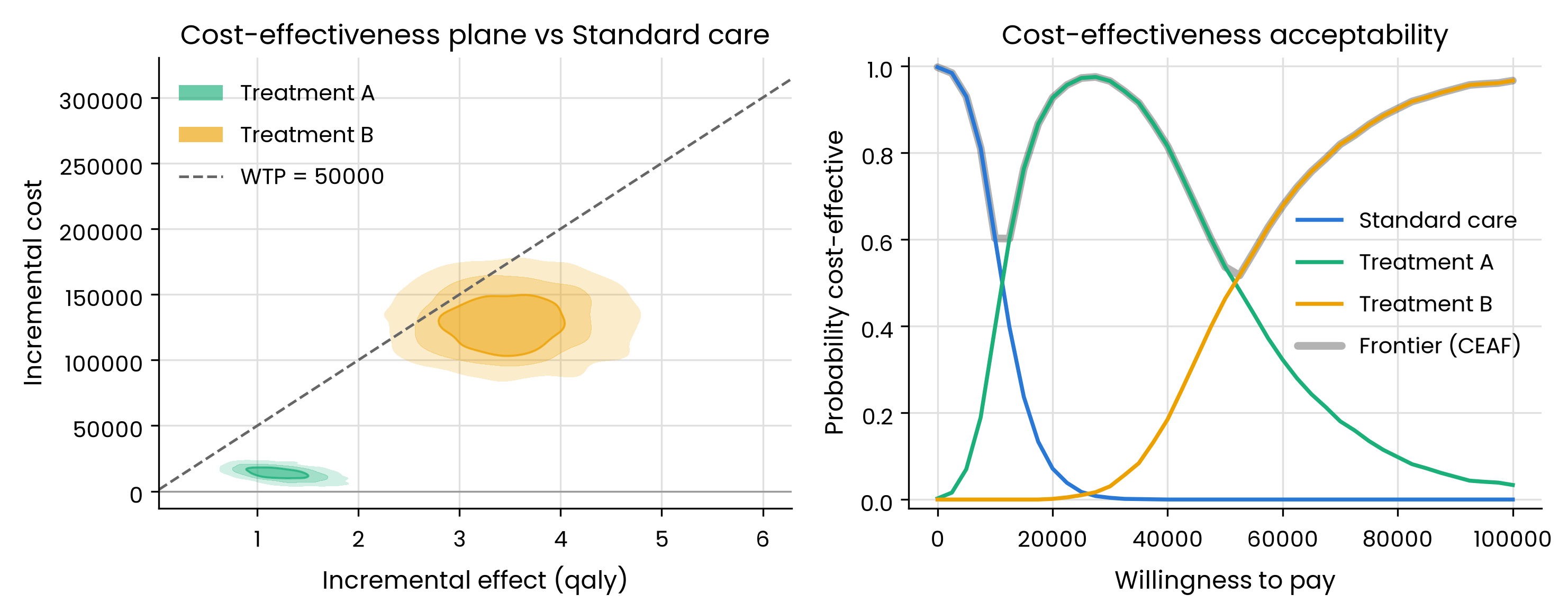
The icer_table orders interventions by cost and reports incremental cost-effectiveness ratios along the efficiency frontier; the status column flags dominated (D) and extended-dominated (ED) interventions. All three interventions lie on the frontier here, with Treatment A entering near 11,000 per quality-adjusted life-year (QALY) and Treatment B near 52,000. plot_ce_plane draws the highest-density regions of every iteration’s incremental cost and effect against standard care, the 50%, 80% and 95% regions of each intervention’s cloud, and plot_ceac reports the share of iterations in which each intervention has the highest net benefit, across a grid of willingness-to-pay thresholds:

grid = np.linspace(0, 100_000, 41)
ceac_df = ceac(outcomes, grid)
ceaf_df = ceaf(outcomes, grid)

fig, axes = plt.subplots(1, 2, figsize=(10, 4))
plot_ce_plane(outcomes, comparator="Standard care", wtp=WTP, ax=axes[0])
plot_ceac(ceac_df, ceaf_df=ceaf_df, ax=axes[1])
fig.tight_layout()

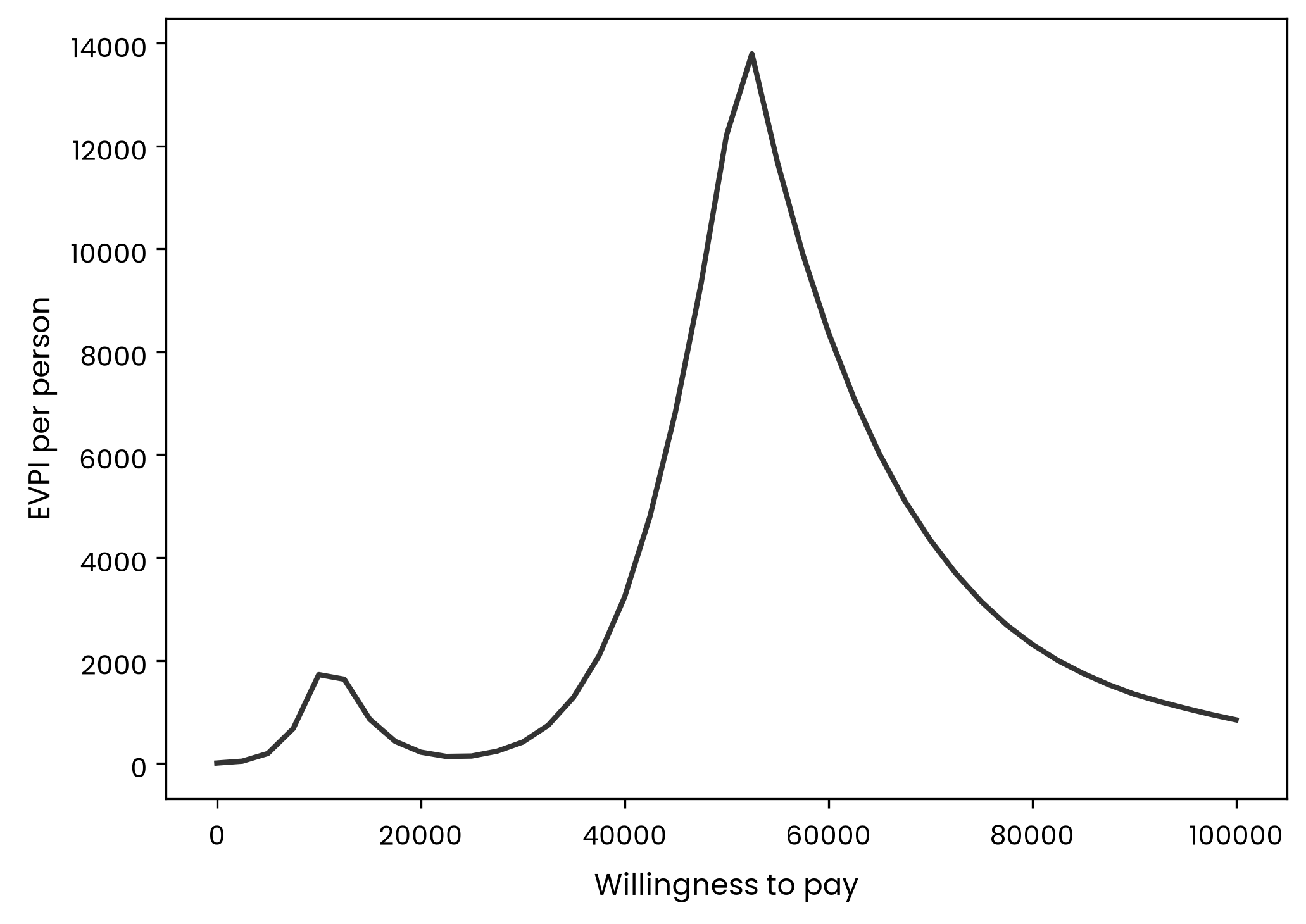
At a willingness-to-pay threshold of 50,000, the acceptability curves cross: the choice between Treatment A and Treatment B is close, so the expected value of perfect information (EVPI) is high there. Swept across the threshold, EVPI peaks near each ICER on the frontier, sharpest where the decision is closest:

evpi_curve = evpi(outcomes, grid)
print(f"EVPI at WTP {WTP:,.0f}: {evpi(outcomes, WTP):,.1f}")

fig2, ax2 = plt.subplots()
ax2.plot(grid, evpi_curve.to_numpy(), color="#333333", lw=2)
ax2.set_xlabel("Willingness to pay")
ax2.set_ylabel("EVPI per person")
fig2.tight_layout()

EVPI at WTP 50,000: 12,205.0

Where to go next

Browse the tutorials

Every tutorial, in the order a reader learns the package, from the standard workflow through the model engines to calibration.

Full pipeline

Parameters, run_psa, cost-effectiveness, and value of information end to end.

Cohort state-transition model

The standard engine, validated against a published result, with the microsimulation engine as the detailed alternative.

Compartmental transmission model

A susceptible-exposed-infectious-recovered vaccination model for infectious-disease cost-effectiveness analysis.

Calibration workflow

Calibrate some parameters, take the rest from the literature, and mix them with mix_draws.

API reference

Every public function, generated from docstrings.

Keywords: cost-effectiveness modeling, cost-effectiveness analysis, value of information, probabilistic sensitivity analysis, health economics, health technology assessment, cohort state-transition model, microsimulation, discrete-event simulation, Bayesian calibration, Python