This tutorial shows how to run the standard probabilistic sensitivity analysis workflow end to end: specify parameters, sample draws, evaluate a model with run_psa, then pass the outcomes to cost-effectiveness and value-of-information analysis. Bring your own outputs covers the analysis functions in more detail; here the focus is the run itself.
Specifying and sampling parameters
The workflow begins by describing each uncertain parameter as a probability distribution and drawing a sample from it. A distribution is specified directly, as with Normal(0.70, 0.10), or from a published mean and standard error, as with Beta.from_mean_se. ParameterSet.sample returns a draw matrix with one row per iteration, and a Spearman rank correlation can be imposed on any pair of parameters to reflect a known dependence.
Each row is one parameter draw. The model is evaluated once per row.
Writing the model as a function
A model is a function that takes the draw matrix and returns Outcomes. The one below is a two-intervention decision tree evaluated over one year. Outcomes.from_wide builds that result from per-intervention cost and effect columns.
run_psa evaluates the model on every draw and keeps each outcome matched to the parameters that produced it, the matching that value-of-information analysis relies on. It runs in parallel by default; this run is small, so sequential=True runs it without that overhead.
from heormodel.run import run_psaoutcomes = run_psa(decision_tree, draws, sequential=True).outcomesoutcomes.summary().round(3)
cost
qaly
intervention
No treatment
4986.265
0.930
Treatment
7505.804
0.951
Analyzing cost-effectiveness and value of information
Nothing from here on is specific to a decision tree: the same icer_table, evpi, and evppi_ranking calls apply to the Outcomes any model produces. The incremental cost-effectiveness ratio (ICER) compares the more effective intervention against its next cheaper alternative,
\[\text{ICER} = \frac{C_1 - C_0}{E_1 - E_0},\]
where \(C\) is expected cost and \(E\) expected effect in quality-adjusted life-years (QALYs). The intervention is cost-effective when its ICER stays below the willingness-to-pay threshold \(\lambda\).
Treatment is the more expensive, more effective intervention. Whether its ICER stays below a given willingness-to-pay threshold, and how much resolving the parameter uncertainty would be worth, are the questions the expected value of perfect information (EVPI) and the per-parameter ranking answer next.
WTP =50_000.0print(f"EVPI at WTP {WTP:,.0f}: {evpi(outcomes, WTP):,.2f}")evppi_ranking(outcomes, draws, WTP).round(2)
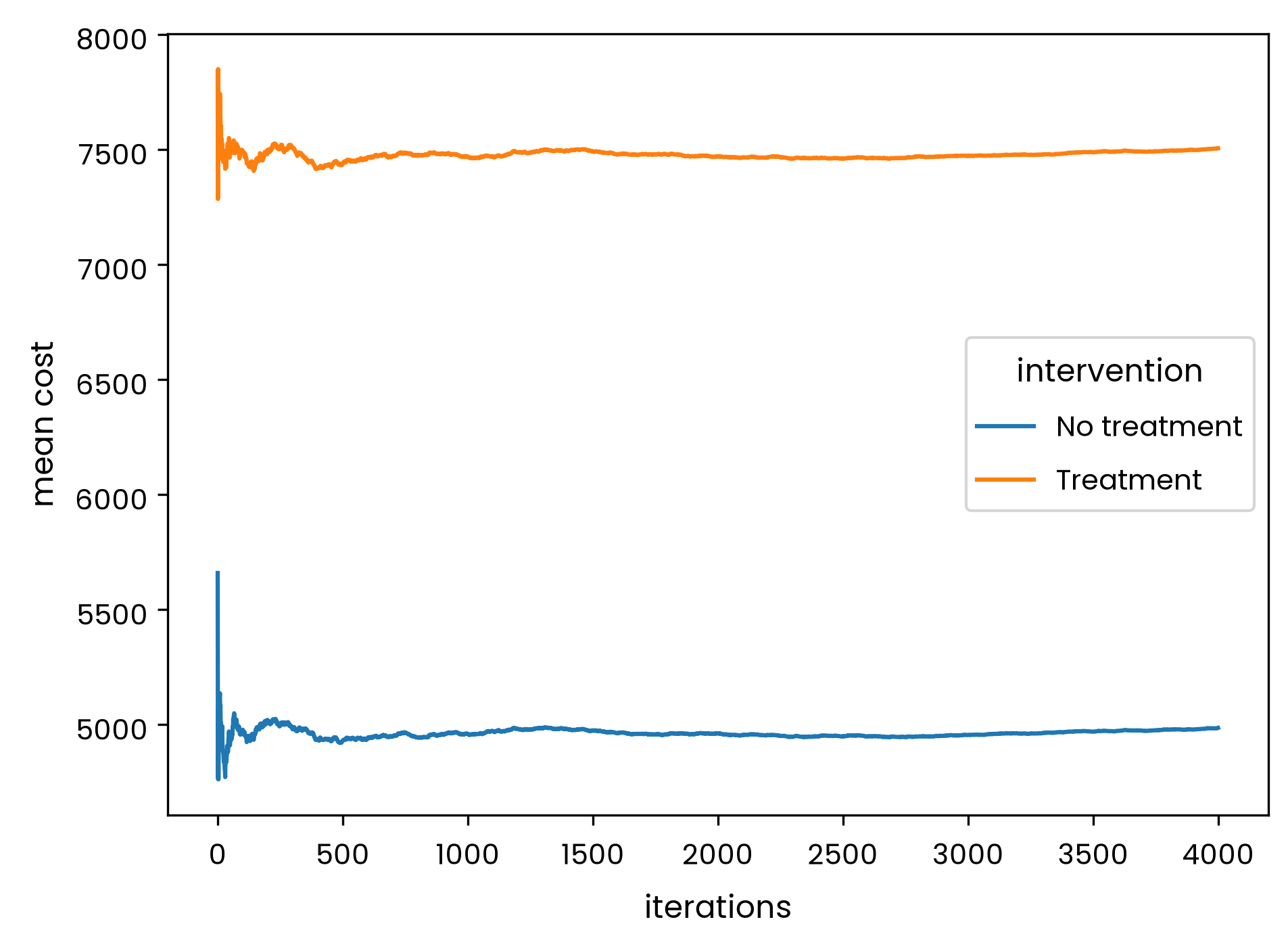
running_means tracks the running mean of an outcome column per intervention as iterations accumulate; flat traces at the right edge suggest the iteration count is adequate for the means (value-of-information estimates typically need more).
from heormodel.run import running_meansrunning_means(outcomes).plot(xlabel="iterations", ylabel="mean cost");
The model engine tutorials cover the model types run_psa can run: cohort state-transition, microsimulation, discrete-event, and compartmental. Next: the value of information tutorial takes the cohort state-transition model from the cohort tutorial through the expected value of perfect, partial perfect, and sample information.
---title: Full pipelinedescription: "Run the standard probabilistic sensitivity analysis end to end: parameters, sampled draws, `run_psa`, then cost-effectiveness and value of information."keywords: [cost-effectiveness analysis, cost-effectiveness modeling, probabilistic sensitivity analysis, PSA, ICER, incremental cost-effectiveness ratio, cost-effectiveness acceptability curve, CEAC, net monetary benefit, health economics, Python]---<!-- colab-badge:start --><a href="https://colab.research.google.com/github/pedroliman/heormodel/blob/main/docs/_notebooks/full-pipeline.ipynb"><img src="https://colab.research.google.com/assets/colab-badge.svg" alt="Open In Colab"></a><!-- colab-badge:end -->This tutorial shows how to run the standard probabilistic sensitivity analysis workflow end to end: specify parameters, sample draws, evaluate a model with `run_psa`, then pass the outcomes to cost-effectiveness and value-of-information analysis. [Bring your own outputs](byo-outputs.qmd) covers the analysis functions in more detail; here the focus is the run itself.## Specifying and sampling parametersThe workflow begins by describing each uncertain parameter as a probability distribution and drawing a sample from it. A distribution is specified directly, as with `Normal(0.70, 0.10)`, or from a published mean and standard error, as with `Beta.from_mean_se`. `ParameterSet.sample` returns a draw matrix with one row per iteration, and a Spearman rank correlation can be imposed on any pair of parameters to reflect a known dependence.```{python}from heormodel.params import Beta, Gamma, Normal, ParameterSetfrom heormodel.run import SeedManagerparams = ParameterSet( {"p_event": Beta.from_mean_se(0.20, 0.03),"rr_treat": Normal(0.70, 0.10),"c_event": Gamma.from_mean_se(25_000, 3_000),"c_treat": Gamma.from_mean_se(4_000, 500),"u_event": Beta.from_mean_se(0.65, 0.05), })seeds = SeedManager(42)draws = params.sample(4_000, seed=seeds.generator())draws.head(3).round(3)```Each row is one parameter draw. The model is evaluated once per row.## Writing the model as a functionA model is a function that takes the draw matrix and returns `Outcomes`. The one below is a two-intervention decision tree evaluated over one year. `Outcomes.from_wide` builds that result from per-intervention cost and effect columns.```{python}import pandas as pdfrom heormodel.models import Outcomesdef decision_tree(d: pd.DataFrame) -> Outcomes: p_treated = d["p_event"] * d["rr_treat"] costs = pd.DataFrame({"No treatment": d["p_event"] * d["c_event"],"Treatment": d["c_treat"] + p_treated * d["c_event"], }) effects = pd.DataFrame({"No treatment": 1- d["p_event"] * (1- d["u_event"]),"Treatment": 1- p_treated * (1- d["u_event"]), })return Outcomes.from_wide(costs, effects)```## Running the probabilistic sensitivity analysis`run_psa` evaluates the model on every draw and keeps each outcome matched to the parameters that produced it, the matching that value-of-information analysis relies on. It runs in parallel by default; this run is small, so `sequential=True` runs it without that overhead.```{python}from heormodel.run import run_psaoutcomes = run_psa(decision_tree, draws, sequential=True).outcomesoutcomes.summary().round(3)```## Analyzing cost-effectiveness and value of informationNothing from here on is specific to a decision tree: the same `icer_table`, `evpi`, and `evppi_ranking` calls apply to the `Outcomes` any model produces. The incremental cost-effectiveness ratio (ICER) compares the more effective intervention against its next cheaper alternative,$$\text{ICER} = \frac{C_1 - C_0}{E_1 - E_0},$$where $C$ is expected cost and $E$ expected effect in quality-adjusted life-years (QALYs). The intervention is cost-effective when its ICER stays below the willingness-to-pay threshold $\lambda$.```{python}import numpy as npfrom heormodel.cea import icer_tablefrom heormodel.voi import evpi, evppi_rankingicer_table(outcomes).round(3)```Treatment is the more expensive, more effective intervention. Whether its ICER stays below a given willingness-to-pay threshold, and how much resolving the parameter uncertainty would be worth, are the questions the expected value of perfect information (EVPI) and the per-parameter ranking answer next.```{python}WTP =50_000.0print(f"EVPI at WTP {WTP:,.0f}: {evpi(outcomes, WTP):,.2f}")evppi_ranking(outcomes, draws, WTP).round(2)```## Checking convergence with running means`running_means` tracks the running mean of an outcome column per intervention as iterations accumulate; flat traces at the right edge suggest the iteration count is adequate for the means (value-of-information estimates typically need more).```{python}from heormodel.run import running_meansrunning_means(outcomes).plot(xlabel="iterations", ylabel="mean cost");```The [model engine tutorials](index.qmd) cover the model types `run_psa` can run: cohort state-transition, microsimulation, discrete-event, and compartmental. Next: the [value of information](voi.qmd) tutorial takes the cohort state-transition model from the [cohort tutorial](mdm-cohort.qmd) through the expected value of perfect, partial perfect, and sample information.