import numpy as np
import pandas as pd
from heormodel.models import CohortSpec, MarkovModel, MicrosimModel, state_occupancy
from heormodel.run import run_psa

STATES = ("healthy", "sick", "dead")
INTERVENTION = "natural_history"
N_CYCLES = 40
TARGET_CYCLES = (8, 16, 28)
BACKGROUND_MORTALITY = 0.01
CALIBRATED = ("p_HS", "p_SD")
BOUNDS = {"p_HS": (0.02, 0.20), "p_SD": (0.05, 0.35)}
TRUTH = {"p_HS": 0.08, "p_SD": 0.15}
SURVEY_SIZE = 1_000
SURVEY_SEED = 20260718
POPULATION = 2_000

def transitions_and_rewards(params, intervention):
    p_HS, p_SD = params["p_HS"], params["p_SD"]
    transition = np.array([
        [1.0 - p_HS - BACKGROUND_MORTALITY, p_HS, BACKGROUND_MORTALITY],
        [0.0, 1.0 - p_SD, p_SD],
        [0.0, 0.0, 1.0],
    ])
    return CohortSpec(transition, np.zeros(3), np.array([1.0, 0.8, 0.0]))

cohort = MarkovModel(
    states=STATES, interventions=(INTERVENTION,),
    transitions_and_rewards=transitions_and_rewards,
    n_cycles=N_CYCLES, cycle_correction="none",
)

def deterministic_prevalence(params):
    occupancy = cohort.trace(pd.Series(params), INTERVENTION)["sick"].to_numpy()
    return np.array([occupancy[cycle] for cycle in TARGET_CYCLES])

def micro_transition(params, intervention, state, attrs, rng):
    p_HS, p_SD = params["p_HS"], params["p_SD"]
    probs = np.zeros((len(state), 3))
    probs[state == 0] = [1.0 - p_HS - BACKGROUND_MORTALITY, p_HS, BACKGROUND_MORTALITY]
    probs[state == 1] = [0.0, 1.0 - p_SD, p_SD]
    probs[state == 2] = [0.0, 0.0, 1.0]
    return probs

def micro_rewards(params, intervention, state, attrs):
    zero = np.zeros(len(state))
return zero, zeroCalibrating a stochastic microsimulation
Calibrate a stochastic microsimulation, carrying its simulation noise into the posterior with a Gaussian process surrogate.

This tutorial calibrates a model that is not only slow but random: an individual-level microsimulation that returns a different result every time it runs. It shows how a Gaussian process surrogate can carry the model’s own variability into the calibration, so the posterior reflects both the sampling error in the data and the simulation noise in the model. The posterior comes out wider than the deterministic calibrations of the earlier tutorials, by an amount that shrinks as the simulated population grows. It walks through examples/calibrate_microsim.py and needs the surrogate extra: uv pip install 'heormodel[surrogate]'.
The three earlier tutorials calibrated a deterministic cohort model, where a parameter set gives one prevalence curve and the only uncertainty is the sample that measured it. A microsimulation is different: it simulates individual people, so a finite population gives a prevalence estimate that changes from run to run. That simulation noise is a second source of uncertainty, separate from the data. Averaging it away would take many runs of an already expensive model, so instead the surrogate learns it: fit a Gaussian process to a few noisy runs, and its predictive spread stands in for the model’s variability without running it again.
Building the microsimulation twin
The microsimulation is the individual-level version of the same three-state model. Every person starts Healthy and moves between Healthy, Sick, and Dead each cycle with the same transition probabilities the cohort model used. Run over a finite population, its Sick-state prevalence approaches the cohort trace as the population grows, so the two are the same model in the limit.
The prevalence comes from an event history: run the microsimulation, then read the share of the population in the Sick state at each target cycle. One run per parameter set gives one noisy reading of the prevalence.
def microsim_prevalence(param_rows, population):
    engine = MicrosimModel.discrete(
        states=STATES, transition_probabilities=micro_transition,
        state_rewards=micro_rewards, population=population, interventions=[INTERVENTION],
        n_cycles=N_CYCLES, cycle_correction="none", initial_state="healthy",
    )
    draws = pd.DataFrame(param_rows)
    draws.index = pd.RangeIndex(len(draws), name="iteration")
    events = run_psa(engine, draws, seed=123, collect="events").events
    occupancy = state_occupancy(
        events, states=STATES, initial_state="healthy", n_individuals=population,
        times=[float(cycle) for cycle in TARGET_CYCLES],
        interventions=[INTERVENTION], iterations=draws.index,
    )
    result = np.zeros((len(draws), len(TARGET_CYCLES)))
    for iteration in range(len(draws)):
        for column, cycle in enumerate(TARGET_CYCLES):
            key = (INTERVENTION, iteration, float(cycle))
            result[iteration, column] = occupancy.loc[key, "sick"]
    return result

check = microsim_prevalence([TRUTH] * 40, population=POPULATION)
pd.DataFrame({
    "deterministic": deterministic_prevalence(TRUTH),
    "microsim_mean": check.mean(0),
    "replicate_sd": check.std(0),
}, index=[f"sick_c{c}" for c in TARGET_CYCLES]).round(4)| deterministic | microsim_mean | replicate_sd | |
|---|---|---|---|
| sick_c8 | 0.2637 | 0.2645 | 0.0089 |
| sick_c16 | 0.1958 | 0.1955 | 0.0096 |
| sick_c28 | 0.0810 | 0.0821 | 0.0070 |
At a population of 2,000 the microsimulation mean matches the cohort prevalence, confirming the two are the same model. The replicate standard deviation, about 0.008, is the run-to-run noise a single simulation carries. This is comparable to the sampling error of the target, so it is not negligible.
Fitting a surrogate to noisy runs
The design is the same 60-point Latin hypercube as the previous tutorial, but each point is now run 10 times, because a noisy model needs repeated runs to reveal both its mean and its spread. The Gaussian process is fit to all 600 noisy readings. Its correlation term captures how the mean prevalence varies with the parameters, and its noise term estimates the replicate variance, so the fitted surrogate carries both. The inputs are scaled to the unit box and the correlation length is bounded, which stops the fit from mistaking the noise for structure.
import warnings
from scipy.stats.qmc import LatinHypercube, scale
from sklearn.exceptions import ConvergenceWarning
from sklearn.gaussian_process import GaussianProcessRegressor
from sklearn.gaussian_process.kernels import RBF, ConstantKernel, WhiteKernel

warnings.filterwarnings("ignore", category=ConvergenceWarning)
low = np.array([BOUNDS[name][0] for name in CALIBRATED])
high = np.array([BOUNDS[name][1] for name in CALIBRATED])
REPLICATES = 10

def to_unit(points):
    return (points - low) / (high - low)

def fit_surrogates(unit_points, targets):
    kernel = (ConstantKernel(1.0, (1e-2, 1e2))
              * RBF([0.3, 0.3], length_scale_bounds=(0.05, 2.0))
              + WhiteKernel(1e-3, (1e-6, 1e-1)))
    return [
        GaussianProcessRegressor(kernel=kernel, normalize_y=True, n_restarts_optimizer=8)
        .fit(unit_points, targets[:, target])
        for target in range(len(TARGET_CYCLES))
    ]
Calibrating with and without the model’s noise
Neural posterior estimation runs against the surrogate. Two simulators are compared, both drawing a sample of 1,000 as the data was measured, but differing in how they treat the model. The survey-only simulator uses the surrogate mean, treating the prevalence surface as known exactly. The survey-and-model simulator draws from the surrogate predictive distribution, so each evaluation carries a draw of the model’s replicate noise alongside the sampling error.
import contextlib, io, logging
logging.getLogger("sbi").setLevel(logging.WARNING)
import torch
from sbi.inference import NPE
from sbi.utils import BoxUniform

POSTERIOR_DRAWS = 3_000
SURROGATE_SIMS = 10_000

def npe_posterior(simulator, observed, prior, sims=SURROGATE_SIMS):
    torch.manual_seed(0)
    theta = prior.sample((sims,))
    inference = NPE(prior=prior, show_progress_bars=False)
    with contextlib.redirect_stdout(io.StringIO()):
        inference.append_simulations(theta, simulator(theta)).train()
    samples = inference.build_posterior().sample(
        (POSTERIOR_DRAWS,), x=torch.tensor(observed, dtype=torch.float32),
        show_progress_bars=False,
    )
    return pd.DataFrame(samples.numpy(), columns=list(CALIBRATED))

def calibrate_at_population(population, prior, observed):
    unit_design = LatinHypercube(d=2, seed=7).random(60)
    design = pd.DataFrame(scale(unit_design, low, high), columns=list(CALIBRATED))
    rows = [row for row in design.to_dict("records") for _ in range(REPLICATES)]
    unit_points = np.repeat(unit_design, REPLICATES, axis=0)
    targets = microsim_prevalence(rows, population=population)
    surrogates = fit_surrogates(unit_points, targets)

    survey_rng = np.random.default_rng(11)
    def survey_only(theta):
        mean = np.column_stack([gp.predict(to_unit(theta.numpy())) for gp in surrogates])
        return torch.tensor(survey_rng.binomial(SURVEY_SIZE, np.clip(mean, 0, 1)) / SURVEY_SIZE,
                            dtype=torch.float32)

    model_rng = np.random.default_rng(12)
    def survey_and_model(theta):
        columns = [gp.predict(to_unit(theta.numpy()), return_std=True) for gp in surrogates]
        mean = np.column_stack([col[0] for col in columns])
        spread = np.column_stack([col[1] for col in columns])
        draw = mean + model_rng.normal(0.0, 1.0, mean.shape) * spread
        return torch.tensor(model_rng.binomial(SURVEY_SIZE, np.clip(draw, 0, 1)) / SURVEY_SIZE,
                            dtype=torch.float32)

    return (npe_posterior(survey_only, observed, prior),
            npe_posterior(survey_and_model, observed, prior))
/home/runner/work/heormodel/heormodel/.venv/lib/python3.12/site-packages/tqdm/auto.py:21: TqdmWarning: IProgress not found. Please update jupyter and ipywidgets. See https://ipywidgets.readthedocs.io/en/stable/user_install.html
from .autonotebook import tqdm as notebook_tqdmThe target is the shared observed reading of the earlier tutorials, so the posteriors are comparable. Calibrating at a population of 2,000 gives the two posteriors.
true_prevalence = deterministic_prevalence(TRUTH)
observed = np.random.default_rng(SURVEY_SEED).binomial(SURVEY_SIZE, true_prevalence) / SURVEY_SIZE
prior = BoxUniform(low=torch.tensor(low, dtype=torch.float32),
                   high=torch.tensor(high, dtype=torch.float32))

survey_only, survey_and_model = calibrate_at_population(POPULATION, prior, observed)
summary = pd.DataFrame({
    "truth": [TRUTH[name] for name in CALIBRATED],
    "survey_only_mean": survey_only.mean().reindex(CALIBRATED).to_numpy(),
    "survey_only_sd": survey_only.std().reindex(CALIBRATED).to_numpy(),
    "model_survey_mean": survey_and_model.mean().reindex(CALIBRATED).to_numpy(),
    "model_survey_sd": survey_and_model.std().reindex(CALIBRATED).to_numpy(),
}, index=list(CALIBRATED))
summary.round(4)| truth | survey_only_mean | survey_only_sd | model_survey_mean | model_survey_sd | |
|---|---|---|---|---|---|
| p_HS | 0.08 | 0.0791 | 0.0057 | 0.0802 | 0.0064 |
| p_SD | 0.15 | 0.1390 | 0.0059 | 0.1399 | 0.0074 |
Both posteriors recover the truth, but the one that carries the model’s noise is wider: its standard deviations exceed the survey-only ones by roughly 10 to 20 percent. The extra width is the simulation noise, propagated by the surrogate into the parameters. Overlaying the marginals shows it.
import matplotlib.pyplot as plt

fig, axes = plt.subplots(1, len(CALIBRATED), figsize=(9, 3.5))
for axis, name in zip(axes, CALIBRATED):
    axis.hist(survey_only[name], bins=40, density=True, alpha=0.5, label="survey only")
    axis.hist(survey_and_model[name], bins=40, density=True, alpha=0.5, label="survey + model")
    axis.axvline(TRUTH[name], color="black", linestyle="--", linewidth=1, label="truth")
    axis.set_xlabel(name)
    axis.set_yticks([])
axes[0].set_ylabel("posterior density")
axes[-1].legend(fontsize=8)
fig.tight_layout()
plt.show()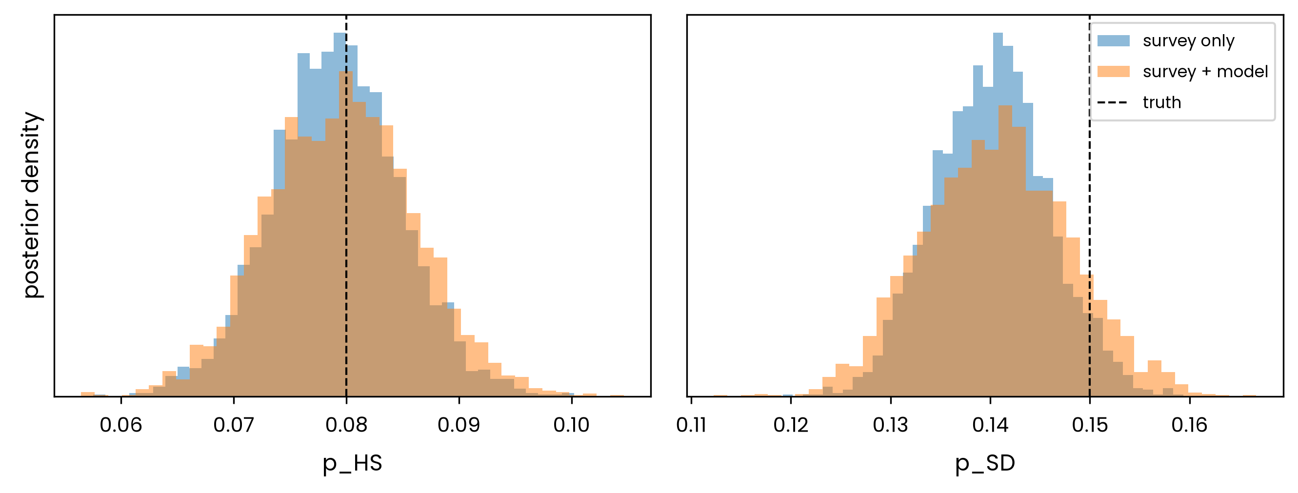
Running the model at a larger population
The extra width is not irreducible: it comes from the finite population each run simulates. Running the microsimulation at a larger population shrinks the replicate noise the surrogate carries, and the posterior narrows toward the survey-only width. Repeating the calibration at a population of 8,000 shows the standard deviation fall back toward the deterministic floor.
_, model_8000 = calibrate_at_population(8_000, prior, observed)
sweep = pd.DataFrame({
    "population_2000_sd": survey_and_model.std().reindex(CALIBRATED).to_numpy(),
    "population_8000_sd": model_8000.std().reindex(CALIBRATED).to_numpy(),
    "survey_only_floor": survey_only.std().reindex(CALIBRATED).to_numpy(),
}, index=list(CALIBRATED))
sweep.round(4)| population_2000_sd | population_8000_sd | survey_only_floor | |
|---|---|---|---|
| p_HS | 0.0064 | 0.0065 | 0.0057 |
| p_SD | 0.0074 | 0.0064 | 0.0059 |
At 8,000 the posterior standard deviation has nearly returned to the survey-only floor, because the replicate noise falls with population like the Monte Carlo error of any microsimulation mean, \(\sigma_\text{rep} \propto 1/\sqrt{N}\), so a four-fold larger population halves it. The width the model’s noise adds is a statement about the simulation budget: with more runs, or larger runs, it shrinks. Reporting it keeps the calibration honest about how much of the posterior uncertainty comes from the data and how much from the model that was run a finite number of times.
This completes the calibration sequence: ABC and simulation-based inference on a deterministic model, both methods on a surrogate, and a stochastic model whose noise the surrogate carries into the posterior.