import numpy as np
import pandas as pd
from heormodel.params import Beta, Gamma, Normal, ParameterSet
from heormodel.run import SeedManager, as_outcomes

WTP = 30_000.0  # sits between the two frontier ratios, so the decision is uncertain
N = 2_000

seed_manager = SeedManager(20260704)
params = ParameterSet(
    {
        "p_response": Beta.from_mean_se(0.35, 0.05),
        "rr_drug": Normal(0.75, 0.08),
        "c_drug": Gamma.from_mean_se(12_000, 1_500),
        "c_monitoring": Gamma.from_mean_se(2_000, 400),
        "u_gain": Beta.from_mean_se(0.12, 0.03),
    },
    correlation={("p_response", "u_gain"): 0.3},
)
draws = params.sample(N, seed=seed_manager.generator())

base_qaly = 8.0
effect_drug = base_qaly + draws["u_gain"] * draws["p_response"] / draws["rr_drug"] * 10
rows = pd.concat([
    pd.DataFrame({"intervention": "Standard care", "iteration": draws.index,
                  "cost": 40_000.0, "qaly": base_qaly}),
    pd.DataFrame({"intervention": "New drug", "iteration": draws.index,
                  "cost": 40_000.0 + draws["c_drug"], "qaly": effect_drug}),
    pd.DataFrame({"intervention": "Drug + monitoring", "iteration": draws.index,
                  "cost": 40_000.0 + draws["c_drug"] + draws["c_monitoring"],
                  "qaly": effect_drug + 0.15 * draws["p_response"]}),
])Bring your own outputs
Take a costs-and-effects table computed elsewhere through cost-effectiveness, value of information, plots, and a reproducibility record, without building a model engine.

This tutorial shows how to take a costs-and-effects table computed outside heormodel, a spreadsheet export or a legacy simulator’s output, and run it through the complete analysis: cost-effectiveness, value of information, plots, and a reproducibility record, without building a model engine. This page walks through examples/byoo_example.py step by step. Install heormodel first: see the overview.
Simulating an external results table
Three interventions compete for a chronic disease: standard of care, a new drug, and drug plus monitoring. A real analysis would load this table from a spreadsheet or a legacy simulator’s output; here it is synthesized from sampled parameters instead, so that the value-of-information results computed later can be traced back to the parameters that drive them.
Converting the table to the standard structure
as_outcomes accepts a DataFrame or a CSV path with intervention, iteration, cost, and effect columns, and returns Outcomes, the structure every analysis function below uses. Converting once here means icer_table, the acceptability curves, the value-of-information estimators, and the plots all take the same Outcomes, regardless of where the numbers originally came from.
outcomes = as_outcomes(rows)
outcomes.summary().round(2)| cost | qaly | |
|---|---|---|
| intervention | ||
| Standard care | 40000.00 | 8.00 |
| New drug | 51985.32 | 8.57 |
| Drug + monitoring | 53981.58 | 8.62 |
Each row gives an intervention’s mean cost and effect across the 2,000 iterations, confirming the table converted into the structure the analysis functions expect.
Running the cost-effectiveness analysis
icer_table orders interventions by cost and reports incremental cost-effectiveness ratios along the efficiency frontier.
from heormodel.cea import ceac, ceaf, icer_table

icer_table(outcomes).round(3)| cost | cost_lo | cost_hi | effect | effect_lo | effect_hi | inc_cost | inc_cost_lo | inc_cost_hi | inc_effect | inc_effect_lo | inc_effect_hi | icer | icer_lo | icer_hi | status | |
|---|---|---|---|---|---|---|---|---|---|---|---|---|---|---|---|---|
| intervention | ||||||||||||||||
| Standard care | 40000.000 | 40000.000 | 40000.000 | 8.000 | 8.000 | 8.000 | NaN | NaN | NaN | NaN | NaN | NaN | NaN | NaN | NaN | ND |
| New drug | 51985.317 | 49355.630 | 54894.988 | 8.572 | 8.265 | 9.041 | 11985.317 | 9355.630 | 14894.988 | 0.572 | 0.265 | 1.041 | 20970.857 | 10962.976 | 47773.334 | ND |
| Drug + monitoring | 53981.578 | 51226.426 | 57018.980 | 8.624 | 8.303 | 9.102 | 1996.261 | 1273.799 | 2852.892 | 0.052 | 0.038 | 0.068 | 38074.078 | 22873.377 | 62353.221 | ND |
The status column marks dominated (D) and extended-dominated (ED) interventions; here all three are non-dominated (ND), and the willingness-to-pay threshold of 30,000 lies between the two frontier incremental cost-effectiveness ratios, so the decision is genuinely uncertain. ceac and ceaf turn that uncertainty into acceptability curves across a grid of thresholds, reused below in the plots and the value-of-information ranking.
grid = np.linspace(0, 80_000, 51)
ceac_df = ceac(outcomes, grid)
ceaf_df = ceaf(outcomes, grid)
Ranking parameters by their value of information
Value-of-information analysis works on the net monetary benefit of each intervention, which places cost and effect on one scale at the willingness-to-pay threshold \(\lambda\),
\[\text{NMB}_d(\theta) = \lambda E_d(\theta) - C_d(\theta).\]
The expected value of perfect information (EVPI) puts a monetary value on resolving every remaining source of uncertainty at once. It is the gain from choosing the best intervention for each parameter draw \(\theta\) rather than the single intervention that is best on average,
\[\text{EVPI} = \mathbb{E}_\theta\!\left[\max_d \text{NMB}_d(\theta)\right] - \max_d \mathbb{E}_\theta\!\left[\text{NMB}_d(\theta)\right].\]
evppi_ranking breaks that value down by parameter instead, so a research budget can target whichever one drives the decision the most; it needs the draw matrix as well as the outcomes, linked to it by the shared iteration index.
from heormodel.voi import evpi, evppi_ranking

print(f"EVPI at WTP {WTP:,.0f}: {evpi(outcomes, WTP):,.1f}")
evppi_ranking(outcomes, draws, WTP).round(1)
EVPI at WTP 30,000: 551.3u_gain 309.9
p_response 94.1
c_monitoring 23.6
c_drug 0.5
rr_drug 0.4
Name: evppi, dtype: float64The ranking is sorted from the highest value downward, so the parameter at the top is the one whose resolution alone would most improve the decision at this threshold, and the first candidate for further data collection.
Plotting the cost-effectiveness plane, acceptability, and tornado
The cost-effectiveness plane draws the highest-density regions of every iteration’s incremental cost and effect against a comparator, so the spread of each intervention’s regions shows the uncertainty that the table’s point estimates alone cannot.
from heormodel.report import plot_ce_plane, plot_ceac, plot_frontier, plot_tornado, tornado_data

plot_ce_plane(outcomes, comparator="Standard care", wtp=WTP);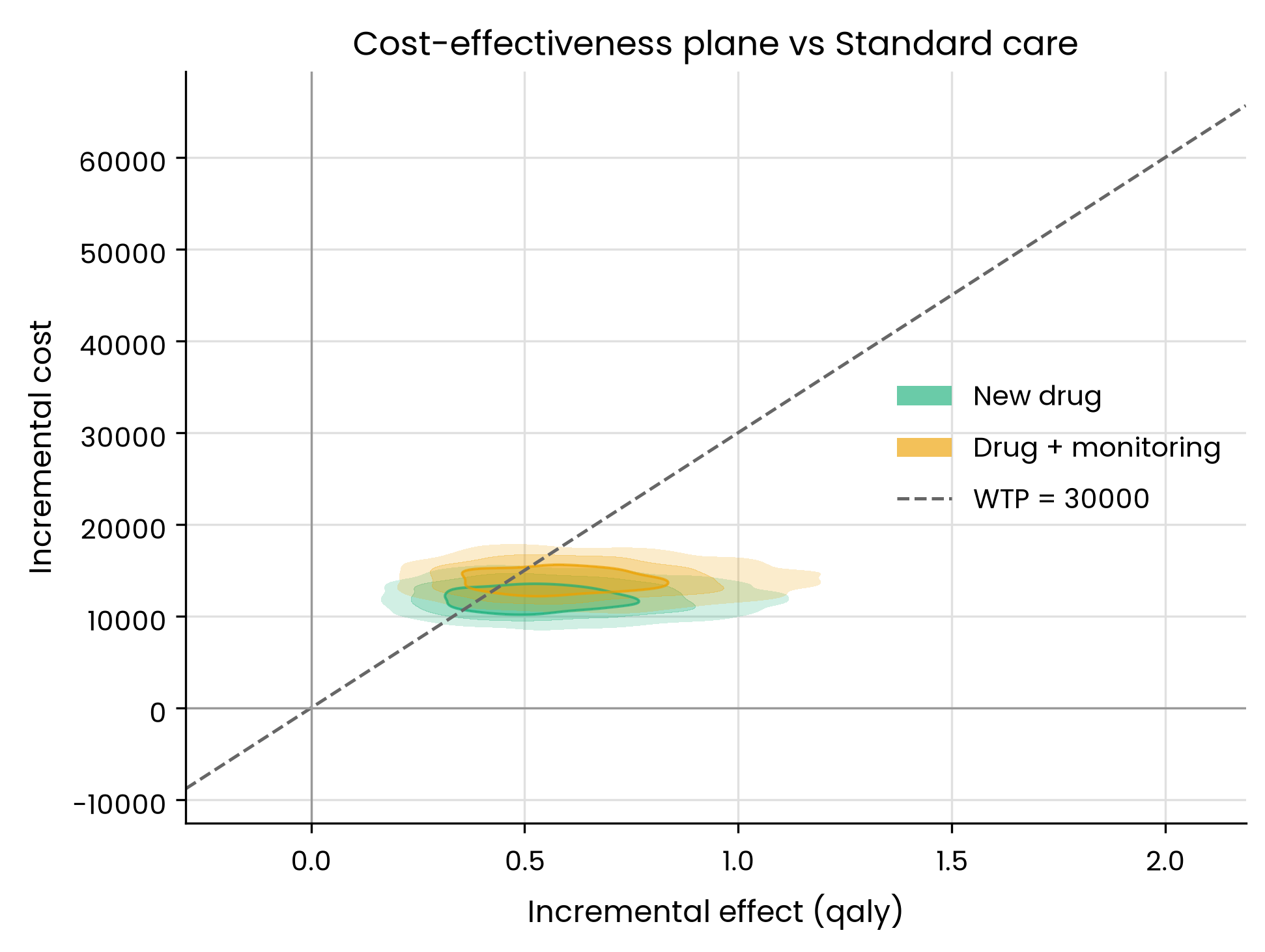
The acceptability curves plot the same probabilities computed above as one line per intervention against the threshold, making the crossover in the decision visible.
plot_ceac(ceac_df, ceaf_df=ceaf_df);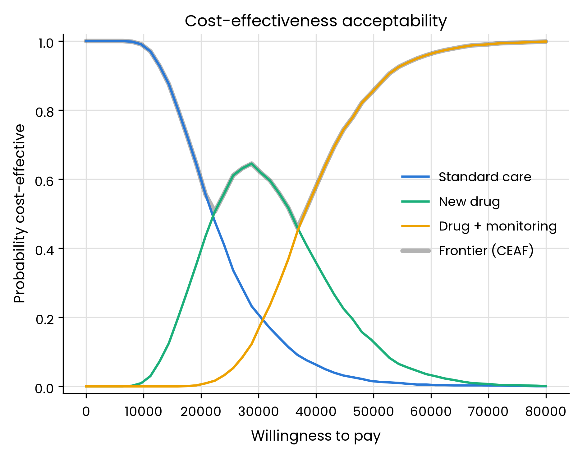
A tornado plot instead breaks down the uncertainty in one comparison, new drug against standard care, by parameter, ranking each by how much it moves the incremental net benefit at the threshold.
td = tornado_data(outcomes, draws, WTP, intervention="New drug", comparator="Standard care")
plot_tornado(td);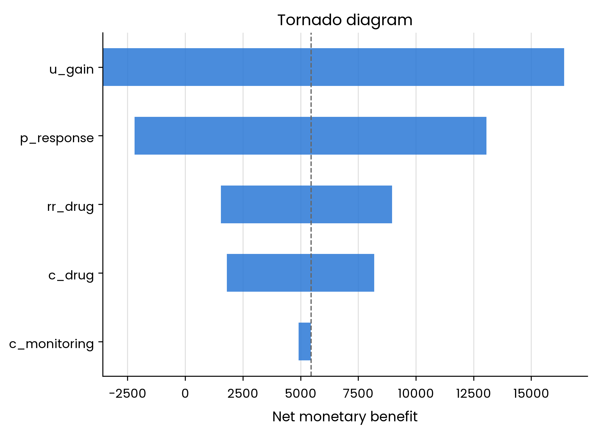
Recording the run for reproducibility
capture_run captures the seed, the parameter specifications, and the outcome shape into a record that saves as JSON and renders as a run report, so a later reviewer can check what produced these numbers without rerunning the analysis.
from heormodel.report import capture_run

record = capture_run(seed=seed_manager, params=params, outcomes=outcomes,
                     note="Bring-your-own-outputs tutorial.")
print(record.to_markdown("heormodel example run report"))
# heormodel example run report
- **Created:** 2026-08-24T06:28:18+00:00
- **Note:** Bring-your-own-outputs tutorial.
- **Root seed entropy:** 20260704
- **Iterations:** 2000
- **Interventions:** Standard care, New drug, Drug + monitoring
## Parameters
| Parameter | Distribution |
|---|---|
| p_response | `Beta(alpha=31.5, beta=58.5)` |
| rr_drug | `Normal(mean_=0.75, sd_=0.08)` |
| c_drug | `Gamma(shape=64, scale=187.5)` |
| c_monitoring | `Gamma(shape=25, scale=80)` |
| u_gain | `Beta(alpha=13.96, beta=102.373)` |
## Software versions
| Package | Version |
|---|---|
| python | 3.12.3 |
| heormodel | 0.7.4 |
| numpy | 2.5.0 |
| scipy | 1.18.0 |
| pandas | 3.0.3 |
| joblib | 1.5.3 |
| scikit-learn | 1.9.0 |
Next: the Markov cohort model builds the standard state-transition model and runs its probabilistic sensitivity analysis through the same analysis functions.