---
title: Calibrating with simulation-based inference
description: "Calibrate the same disease model with neural posterior estimation, a form of simulation-based inference, and recover the same posterior as approximate Bayesian computation."
---
<!-- colab-badge:start -->
<a href="https://colab.research.google.com/github/pedroliman/heormodel/blob/main/docs/_notebooks/calibrate-sbi.ipynb"><img src="https://colab.research.google.com/assets/colab-badge.svg" alt="Open In Colab"></a>
<!-- colab-badge:end -->
This tutorial calibrates the same disease model as the [ABC tutorial](calibrate-abc.qmd), to the same target, with a different method: [neural posterior estimation](https://sbi-dev.github.io/sbi/latest/), a form of simulation-based inference (SBI). It shows that the two methods reach the same posterior when both run against the model directly, so the choice of method is separate from the model it runs on. It walks through [`examples/calibrate_sbi.py`](https://github.com/pedroliman/heormodel/blob/main/examples/calibrate_sbi.py) and needs the surrogate extra, which supplies the inference package: `uv pip install 'heormodel[surrogate]'`.
Simulation-based inference learns the relationship between parameters and outputs from simulated pairs, then reads the posterior off that learned relationship. Neural posterior estimation is one form: it trains a flexible model $q_\phi(\theta \mid x)$ of the distribution of parameters $\theta$ given an output $x$, on pairs drawn from the prior, then evaluates it at the observed target so that $q_\phi(\theta \mid x_\text{obs})$ approximates the posterior. Unlike approximate Bayesian computation, which discards most of its runs by rejecting them, it uses every simulated pair to fit the estimator, and unlike a likelihood-based method it never requires the likelihood to be written down.
## Specifying the model and the target
The model and the target are the same as in the ABC tutorial: a three-state cohort model calibrated to the Sick-state prevalence at three cycles, measured in a sample of 1,000 people, generated from known truth with a fixed seed so both tutorials share the identical observed reading.
```{python}
import numpy as np
import pandas as pd
from heormodel.models import CohortSpec, MarkovModel

STATES = ("healthy", "sick", "dead")
INTERVENTION = "natural_history"
N_CYCLES = 40
TARGET_CYCLES = (8, 16, 28)
BACKGROUND_MORTALITY = 0.01
CALIBRATED = ("p_HS", "p_SD")
BOUNDS = {"p_HS": (0.02, 0.20), "p_SD": (0.05, 0.35)}
TRUTH = {"p_HS": 0.08, "p_SD": 0.15}
SURVEY_SIZE = 1_000
SURVEY_SEED = 20260718

def transitions_and_rewards(params, intervention):
    p_HS, p_SD = params["p_HS"], params["p_SD"]
    transition = np.array([
        [1.0 - p_HS - BACKGROUND_MORTALITY, p_HS, BACKGROUND_MORTALITY],
        [0.0, 1.0 - p_SD, p_SD],
        [0.0, 0.0, 1.0],
    ])
    return CohortSpec(transition, np.zeros(3), np.array([1.0, 0.8, 0.0]))

engine = MarkovModel(
    states=STATES, interventions=(INTERVENTION,),
    transitions_and_rewards=transitions_and_rewards,
    n_cycles=N_CYCLES, cycle_correction="none",
)
model_runs = {"count": 0}

def prevalence(params):
    """Sick-state prevalence at the target cycles; one model run, counted."""
    model_runs["count"] += 1
    occupancy = engine.trace(pd.Series(params), INTERVENTION)["sick"].to_numpy()
    return np.array([occupancy[cycle] for cycle in TARGET_CYCLES])

true_prevalence = prevalence(TRUTH)
observed = np.random.default_rng(SURVEY_SEED).binomial(SURVEY_SIZE, true_prevalence) / SURVEY_SIZE
observed.round(4)
```
The observed reading matches the one the ABC tutorial calibrated against.
## Training the density estimator
The prior is a box over the two parameters. The simulator draws a parameter set, runs the model, and returns a sample of the resulting prevalence, so each training pair carries the same sampling error the data has. Neural posterior estimation trains on 10,000 such pairs. Every pair is a model run, which is the cost this method carries: the density estimator needs a large training set to learn the mapping across the whole prior.
```{python}
import contextlib, io, logging
logging.getLogger("sbi").setLevel(logging.WARNING)  # quiet sbi's per-epoch logging

import torch
from sbi.inference import NPE
from sbi.utils import BoxUniform

low = np.array([BOUNDS[name][0] for name in CALIBRATED])
high = np.array([BOUNDS[name][1] for name in CALIBRATED])
torch.manual_seed(0)
survey_rng = np.random.default_rng(11)
prior = BoxUniform(low=torch.tensor(low, dtype=torch.float32),
                   high=torch.tensor(high, dtype=torch.float32))

def simulator(theta):
    means = np.array([prevalence(dict(zip(CALIBRATED, row))) for row in theta.numpy()])
    survey = survey_rng.binomial(SURVEY_SIZE, means) / SURVEY_SIZE
    return torch.tensor(survey, dtype=torch.float32)

model_runs["count"] = 0
theta = prior.sample((10_000,))
x = simulator(theta)
print(f"{model_runs['count']} model runs to build the training set")

inference = NPE(prior=prior, show_progress_bars=False)
with contextlib.redirect_stdout(io.StringIO()):  # quiet sbi's training progress print
    inference.append_simulations(theta, x).train()
neural_posterior = inference.build_posterior()
```
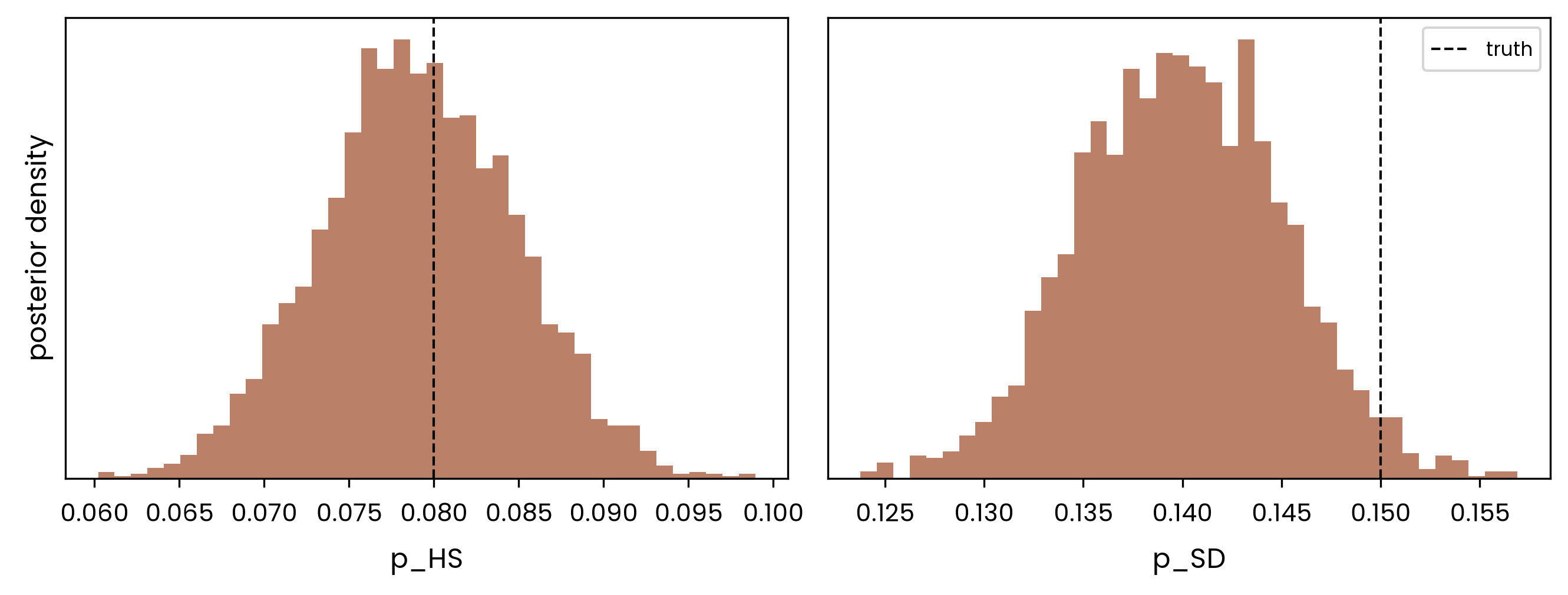
The trained estimator is amortized: it represents the posterior for any target, not only the one observed. Conditioning it on the observed reading returns the posterior without further model runs.
```{python}
samples = neural_posterior.sample(
    (3_000,), x=torch.tensor(observed, dtype=torch.float32), show_progress_bars=False
)
posterior = pd.DataFrame(samples.numpy(), columns=list(CALIBRATED))
summary = pd.DataFrame({
    "truth": [TRUTH[name] for name in CALIBRATED],
    "posterior_mean": posterior.mean().reindex(CALIBRATED).to_numpy(),
    "posterior_sd": posterior.std().reindex(CALIBRATED).to_numpy(),
}, index=list(CALIBRATED))
summary.round(4)
```
The posterior means recover the truth, and the standard deviations match the ABC posterior to within about 0.001. The two methods, given the same model and the same target, agree on both the location and the spread of the posterior.
```{python}
import matplotlib.pyplot as plt

fig, axes = plt.subplots(1, len(CALIBRATED), figsize=(9, 3.5))
for axis, name in zip(axes, CALIBRATED):
    axis.hist(posterior[name], bins=40, density=True, alpha=0.6, color="#8c2d04")
    axis.axvline(TRUTH[name], color="black", linestyle="--", linewidth=1, label="truth")
    axis.set_xlabel(name)
    axis.set_yticks([])
axes[0].set_ylabel("posterior density")
axes[-1].legend(fontsize=8)
fig.tight_layout()
plt.show()
```
The training set cost 10,000 model runs, the same order as the ABC run in the previous tutorial. Neither method is cheap in model runs, because both learn the posterior by running the model across the prior. When the model is slow, that budget is the obstacle. The [next tutorial](surrogate-calibration.qmd) removes it by fitting a fast surrogate on a few dozen runs and inferring against the surrogate, with both methods, at a fraction of the cost.