---
title: Surrogate-accelerated calibration
description: "Fit a fast surrogate of an expensive model on a small design, then calibrate against the surrogate instead of the model."
---
<!-- colab-badge:start -->
<a href="https://colab.research.google.com/github/pedroliman/heormodel/blob/main/docs/_notebooks/surrogate-calibration.ipynb"><img src="https://colab.research.google.com/assets/colab-badge.svg" alt="Open In Colab"></a>
<!-- colab-badge:end -->
This tutorial shows how to calibrate a model too slow to run the thousands of times direct inference needs. The approach moves that cost up front: run the model a few dozen times over a fixed design, fit a fast surrogate (a metamodel) that approximates its output, and run the inference against the surrogate instead of the model. The first two calibration tutorials each ran the model directly, which needed at least a few thousand runs; a surrogate replaces almost all of them.
The surrogate here is a [Gaussian process](https://scikit-learn.org/stable/modules/gaussian_process.html) (GP). A Gaussian process is used because it is fast to fit and reports its own uncertainty, so a draw from it carries the approximation error forward, which a single-point prediction would hide. We fit one GP per target on a few dozen model runs, then calibrate against it twice, once with approximate Bayesian computation (ABC) and once with neural posterior estimation, and check that each recovers the known parameters.
This tutorial builds on the [ABC](calibrate-abc.qmd) and [simulation-based inference](calibrate-sbi.qmd) tutorials, walks through [`examples/surrogate_calibration.py`](https://github.com/pedroliman/heormodel/blob/main/examples/surrogate_calibration.py), and needs both extras: `uv pip install 'heormodel[calibration,surrogate]'`.
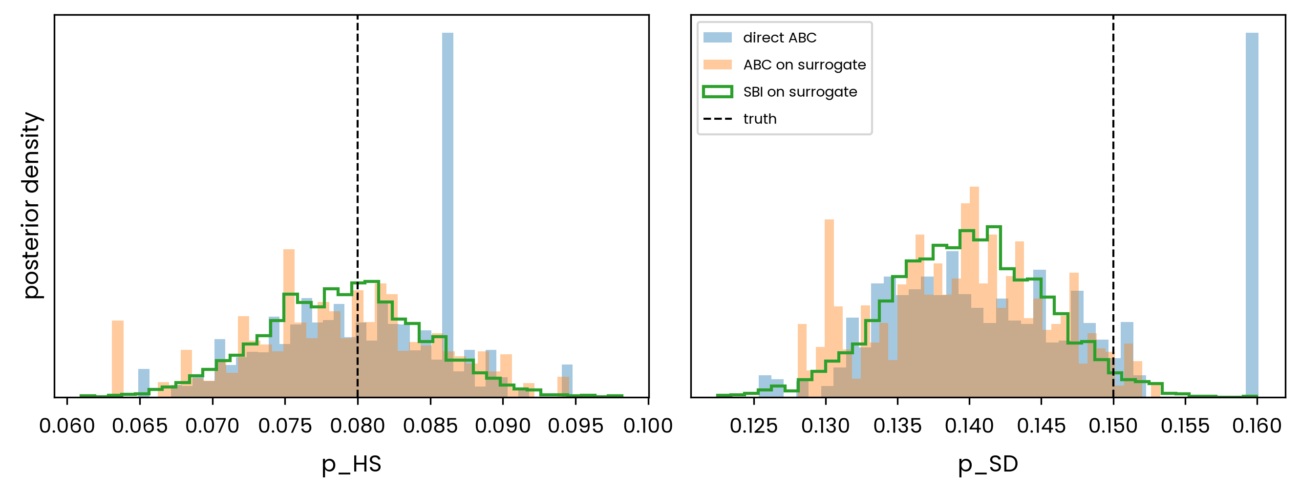
The tutorial makes two points. The surrogate is faithful, so inference against it reproduces the direct posterior. And the two inference methods, run on the same surrogate, agree, so the method and the surrogate are independent choices.
## Specifying the model and the target
The model and the target are those of the previous two tutorials: a three-state cohort model calibrated to the Sick-state prevalence at three cycles, measured in a sample of 1,000 people, generated from known truth with the shared seed.
```{python}
import numpy as np
import pandas as pd
from heormodel.models import CohortSpec, MarkovModel

STATES = ("healthy", "sick", "dead")
INTERVENTION = "natural_history"
N_CYCLES = 40
TARGET_CYCLES = (8, 16, 28)
TARGET_LABELS = [f"sick_c{cycle}" for cycle in TARGET_CYCLES]
BACKGROUND_MORTALITY = 0.01
CALIBRATED = ("p_HS", "p_SD")
BOUNDS = {"p_HS": (0.02, 0.20), "p_SD": (0.05, 0.35)}
TRUTH = {"p_HS": 0.08, "p_SD": 0.15}
SURVEY_SIZE = 1_000
SURVEY_SEED = 20260718

def transitions_and_rewards(params, intervention):
    p_HS, p_SD = params["p_HS"], params["p_SD"]
    transition = np.array([
        [1.0 - p_HS - BACKGROUND_MORTALITY, p_HS, BACKGROUND_MORTALITY],
        [0.0, 1.0 - p_SD, p_SD],
        [0.0, 0.0, 1.0],
    ])
    return CohortSpec(transition, np.zeros(3), np.array([1.0, 0.8, 0.0]))

engine = MarkovModel(
    states=STATES, interventions=(INTERVENTION,),
    transitions_and_rewards=transitions_and_rewards,
    n_cycles=N_CYCLES, cycle_correction="none",
)
model_runs = {"count": 0}

def prevalence(params):
    """Sick-state prevalence at the target cycles; one model run, counted."""
    model_runs["count"] += 1
    occupancy = engine.trace(pd.Series(params), INTERVENTION)["sick"].to_numpy()
    return np.array([occupancy[cycle] for cycle in TARGET_CYCLES])

def draw_survey(prevalences, rng):
    return rng.binomial(SURVEY_SIZE, np.clip(prevalences, 0, 1)) / SURVEY_SIZE

true_prevalence = prevalence(TRUTH)
observed = draw_survey(true_prevalence, np.random.default_rng(SURVEY_SEED))
epsilon = 0.5 * float(np.sqrt((true_prevalence * (1 - true_prevalence) / SURVEY_SIZE).sum()))
observed.round(4)
```
## Fitting a Gaussian process surrogate
The design is a Latin hypercube sample of 60 points over the two parameters, chosen because it spreads points evenly through the parameter box rather than clustering them as independent uniform draws would. Sixty points is a deliberately small budget, to show that the surrogate fits this two-parameter model well from only a few dozen runs.
```{python}
import warnings
from scipy.stats.qmc import LatinHypercube, scale
from sklearn.exceptions import ConvergenceWarning
from sklearn.gaussian_process import GaussianProcessRegressor
from sklearn.gaussian_process.kernels import RBF, ConstantKernel, WhiteKernel

warnings.filterwarnings("ignore", category=ConvergenceWarning)  # cosmetic; hold-out confirms fit
low = np.array([BOUNDS[name][0] for name in CALIBRATED])
high = np.array([BOUNDS[name][1] for name in CALIBRATED])

model_runs["count"] = 0
design = pd.DataFrame(scale(LatinHypercube(d=2, seed=7).random(60), low, high),
                     columns=list(CALIBRATED))
design_targets = np.array([prevalence(row) for row in design.to_dict("records")])
design_runs = model_runs["count"]
print(f"{design_runs} model runs for the design")
```
A Gaussian process regresses each target on the two parameters, one process per target. At any parameter point it returns not a single number but a predictive distribution, a mean and a variance, $f(x) \sim \mathcal{N}\big(\mu(x),\, \sigma^2(x)\big)$, with the variance widening away from the design points. That is why it suits a small design of a smooth function: it interpolates the runs it has and reports how uncertain it is everywhere else. For the full treatment, see the [GP regression chapter](https://bookdown.org/rbg/surrogates/chap5.html) and the [scikit-learn documentation on GPs](https://scikit-learn.org/stable/modules/gaussian_process.html).
```{python}
kernel = ConstantKernel(1.0) * RBF([0.1, 0.1]) + WhiteKernel(1e-6, (1e-10, 1e-2))
surrogates = [
    GaussianProcessRegressor(kernel=kernel, normalize_y=True, n_restarts_optimizer=5)
    .fit(design.to_numpy(), design_targets[:, target])
    for target in range(len(TARGET_LABELS))
]
```
A surrogate is only useful if it is accurate where the design did not place points, so it must be checked against model runs that were not in its design. Predicting 300 fresh points and comparing to the model gives the root-mean-square error per target.
```{python}
holdout = scale(LatinHypercube(d=2, seed=99).random(300), low, high)
holdout_targets = np.array([prevalence(dict(zip(CALIBRATED, row))) for row in holdout])
predicted = np.column_stack([gp.predict(holdout) for gp in surrogates])
rmse = np.sqrt(((predicted - holdout_targets) ** 2).mean(axis=0))
print("hold-out RMSE per target:", rmse.round(5))
```
The error is on the order of 0.0001, so at this scale the surrogate is indistinguishable from the model and inference against it should find the same posterior.
## Calibrating against the surrogate with both methods
Both methods now use the surrogate as their simulator. Each evaluation predicts the prevalence from the Gaussian process and draws a sample of it, so the surrogate simulators carry the same sampling error the direct calibrations did, without running the model.
```{python}
import os
os.environ["ABC_LOG_LEVEL"] = "WARNING"
import logging
logging.getLogger("sbi").setLevel(logging.WARNING)

from heormodel.calibrate import abc_calibrate
from heormodel.params import Uniform

priors = {name: Uniform(*BOUNDS[name]) for name in CALIBRATED}
observed_map = dict(zip(TARGET_LABELS, observed))

abc_surrogate_rng = np.random.default_rng(2024)

def surrogate_prevalence(params):
    point = np.array([[params[name] for name in CALIBRATED]])
    return np.clip([gp.predict(point)[0] for gp in surrogates], 0, 1)

def abc_surrogate_simulator(params):
    drawn = draw_survey(surrogate_prevalence(params), abc_surrogate_rng)
    return dict(zip(TARGET_LABELS, drawn))

abc_surrogate = abc_calibrate(
    abc_surrogate_simulator, priors=priors, observed=observed_map,
    population_size=400, max_populations=15, min_epsilon=epsilon, n_posterior=3_000, seed=1,
).posterior
```
Neural posterior estimation trains on 10,000 pairs, all from the surrogate, so this stage runs the model zero more times.
```{python}
import contextlib, io, torch
from sbi.inference import NPE
from sbi.utils import BoxUniform

torch.manual_seed(0)
sbi_rng = np.random.default_rng(11)
prior = BoxUniform(low=torch.tensor(low, dtype=torch.float32),
                   high=torch.tensor(high, dtype=torch.float32))

def sbi_surrogate_simulator(theta):
    mean = np.column_stack([gp.predict(theta.numpy()) for gp in surrogates])
    return torch.tensor(draw_survey(mean, sbi_rng), dtype=torch.float32)

theta = prior.sample((10_000,))
inference = NPE(prior=prior, show_progress_bars=False)
with contextlib.redirect_stdout(io.StringIO()):
    inference.append_simulations(theta, sbi_surrogate_simulator(theta)).train()
sbi_surrogate = pd.DataFrame(
    inference.build_posterior().sample(
        (3_000,), x=torch.tensor(observed, dtype=torch.float32), show_progress_bars=False
    ).numpy(),
    columns=list(CALIBRATED),
)
```
## Comparing against a direct calibration
To confirm the surrogate did not distort the answer, run ABC once more against the model itself, the calibration of the first tutorial.
```{python}
reference_rng = np.random.default_rng(2024)

def reference_simulator(params):
    return dict(zip(TARGET_LABELS, draw_survey(prevalence(params), reference_rng)))

model_runs["count"] = 0
reference = abc_calibrate(
    reference_simulator, priors=priors, observed=observed_map,
    population_size=400, max_populations=15, min_epsilon=epsilon, n_posterior=3_000, seed=1,
).posterior
reference_runs = model_runs["count"]
```
The three posteriors agree on the location and the spread of both parameters.
```{python}
def describe(name, draws):
    return {f"{name}_mean": draws.mean().reindex(CALIBRATED).to_numpy(),
            f"{name}_sd": draws.std().reindex(CALIBRATED).to_numpy()}

summary = pd.DataFrame({
    "truth": [TRUTH[name] for name in CALIBRATED],
    **describe("direct", reference),
    **describe("abc_surr", abc_surrogate),
    **describe("sbi_surr", sbi_surrogate),
}, index=list(CALIBRATED))
summary.round(4)
```
The surrogate posteriors, from either method, overlap the direct posterior and center on the truth.
```{python}
import matplotlib.pyplot as plt

fig, axes = plt.subplots(1, len(CALIBRATED), figsize=(9, 3.5))
for axis, name in zip(axes, CALIBRATED):
    axis.hist(reference[name], bins=40, density=True, alpha=0.4, label="direct ABC")
    axis.hist(abc_surrogate[name], bins=40, density=True, alpha=0.4, label="ABC on surrogate")
    axis.hist(sbi_surrogate[name], bins=40, density=True, histtype="step",
              linewidth=1.5, label="SBI on surrogate")
    axis.axvline(TRUTH[name], color="black", linestyle="--", linewidth=1, label="truth")
    axis.set_xlabel(name)
    axis.set_yticks([])
axes[0].set_ylabel("posterior density")
axes[-1].legend(fontsize=7)
fig.tight_layout()
plt.show()
```
Next: the [microsimulation tutorial](calibrate-microsim.qmd) calibrates a model whose runs are not only slow but random, where the surrogate also carries the model's own variability into the posterior.