import numpy as np
import pandas as pd
from heormodel.models import CohortSpec, MarkovModel
from heormodel.params import Beta, Gamma, LogNormal, ParameterSet
from heormodel.run import SeedManager, run_psa

STATES = ("H", "S1", "S2", "D")
INTERVENTIONS = ("Standard of care", "Intervention A", "Intervention B", "Intervention AB")
WTP = 100_000.0

def r2p(rate):  # rate to per-cycle probability
    return 1.0 - np.exp(-np.asarray(rate))

def model(p, intervention):
    p_HS1, p_S1H, p_S1S2 = r2p(p["r_HS1"]), r2p(p["r_S1H"]), r2p(p["r_S1S2"])
    p_HD, p_S1D, p_S2D = r2p(p["r_HD"]), r2p(p["r_HD"] * p["hr_S1"]), r2p(p["r_HD"] * p["hr_S2"])
    prog = r2p(p["r_S1S2"] * p["hr_S1S2_trtB"]) if "B" in intervention else p_S1S2
    P = np.zeros((4, 4))
    P[0, 0], P[0, 1], P[0, 3] = (1 - p_HD) * (1 - p_HS1), (1 - p_HD) * p_HS1, p_HD
    P[1, 0], P[1, 2], P[1, 3] = (1 - p_S1D) * p_S1H, (1 - p_S1D) * prog, p_S1D
    P[1, 1] = (1 - p_S1D) * (1 - p_S1H - prog)
    P[2, 2], P[2, 3], P[3, 3] = 1 - p_S2D, p_S2D, 1.0
    add = {"Standard of care": 0.0, "Intervention A": p["c_trtA"],
           "Intervention B": p["c_trtB"], "Intervention AB": p["c_trtA"] + p["c_trtB"]}[intervention]
    cost = np.array([p["c_H"], p["c_S1"] + add, p["c_S2"] + add, 0.0])
    u_s1 = p["u_trtA"] if intervention in ("Intervention A", "Intervention AB") else p["u_S1"]
    return CohortSpec(P, cost, np.array([p["u_H"], u_s1, p["u_S2"], 0.0]))

engine = MarkovModel(states=STATES, interventions=INTERVENTIONS, transitions_and_rewards=model,
                            n_cycles=75, initial_state="H", cycle_correction="simpson")

params = ParameterSet({
    "r_HD": Gamma(20, 1/10000), "r_HS1": Gamma(30, 1/200), "r_S1H": Gamma(60, 1/120),
    "r_S1S2": Gamma(84, 1/800), "hr_S1": LogNormal(np.log(3), 0.01),
    "hr_S2": LogNormal(np.log(10), 0.02), "hr_S1S2_trtB": LogNormal(np.log(0.6), 0.02),
    "c_H": Gamma(100, 20.0), "c_S1": Gamma(177.8, 22.5), "c_S2": Gamma(225, 66.7),
    "c_trtA": Gamma(73.5, 163.3), "c_trtB": Gamma(86.2, 150.8),
    "u_H": Beta(200, 3), "u_S1": Beta(130, 45), "u_S2": Beta(230, 230), "u_trtA": Beta(300, 15),
})
draws = params.sample(10_000, seed=SeedManager(20260705).generator())
outcomes = run_psa(engine, draws).outcomesValue of information
Run the value-of-information workflow: expected value of perfect, partial perfect, and sample information.
Keywords
value of information, VOI, EVPI, EVPPI, EVSI, expected value of perfect information, expected value of partial perfect information, expected value of sample information, health economics, Python

This tutorial shows how to run the full value-of-information workflow: expected value of perfect information (EVPI), of partial perfect information (EVPPI), and of sample information (EVSI), on the Sick-Sicker cohort state-transition model built in the cohort state-transition tutorial. The full script is examples/voi_tutorial.py.
Specifying the decision model
The model is the four-state, four-intervention Sick-Sicker model from the cohort state-transition tutorial: standard of care, Intervention A (raises the Sick-state utility), Intervention B (slows progression from Sick to Sicker), and the combination AB, evaluated over 75 annual cycles. See that tutorial for the state-transition model and the parameter distributions; the code below reconstructs both so this page runs on its own.
Value-of-information estimates need more draws than a mean cost-effectiveness estimate does, so this run uses 10,000 iterations against the cohort tutorial’s 1,000.
Calculating the expected value of perfect information (EVPI)
EVPI is the difference between a decision made with perfect information and one made with current information, an upper bound on the value of any research.
from heormodel.voi import evpi

evpi(outcomes, WTP)2802.51210525009Ranking parameters with EVPPI
The expected value of partial perfect information (EVPPI) is the value of resolving one parameter, or a group, while the rest stay uncertain. It replaces the inner maximization of EVPI with an expectation taken over only the parameter of interest \(\phi\),
\[\text{EVPPI}_\phi = \mathbb{E}_\phi\!\left[\max_d \mathbb{E}_{\theta \mid \phi}\, \text{NMB}_d\right] - \max_d \mathbb{E}_\theta\, \text{NMB}_d,\]
so it identifies which parameters drive the decision uncertainty. evppi_ranking sweeps each of the model’s 16 parameters and sorts them into a research priority list.
from heormodel.voi import evppi, evppi_ranking

ranking = evppi_ranking(outcomes, draws, WTP)
ranking.round(1)
u_S1 823.4
c_trtA 366.8
c_trtB 66.0
u_H 2.2
hr_S2 1.5
r_S1S2 1.4
hr_S1S2_trtB 0.0
hr_S1 0.0
c_H 0.0
c_S2 0.0
u_trtA 0.0
r_S1H 0.0
r_HS1 0.0
r_HD 0.0
c_S1 0.0
u_S2 0.0
Name: evppi, dtype: float64u_S1, the Sick-state utility under standard of care, dominates the ranking: Intervention A’s entire benefit is raising that utility to u_trtA, so whether the true u_S1 is already close to u_trtA decides whether Intervention A is worth its cost. The two treatment costs c_trtA and c_trtB follow, with everything else contributing almost nothing at this threshold. The spline metamodel used by default handles one parameter at a time well; method="gp" (a Gaussian process) suits groups of many parameters evaluated jointly.
Expected value of sample information (EVSI)
EVSI is the value of a study of finite sample size, the practical counterpart to the perfect-information measures above, which assume a parameter is resolved exactly. Since u_S1 drives the ranking, consider a preference-based utility survey of Sick patients, each reporting a health-utility score with the sampling standard deviation typical of an instrument like the EQ-5D-5L in a chronic-disease population. simulate_summaries draws one survey summary per parameter draw from its true u_S1, and evsi_regression computes the value from the fitted conditional means.
from heormodel.voi import evsi_regression, simulate_summaries

PATIENT_SD = 0.20  # per-patient sd of a preference-based utility instrument
n_survey = 400
tau = PATIENT_SD / np.sqrt(n_survey)
summaries = simulate_summaries(
    draws, lambda row, r: {"ubar": row["u_S1"] + r.normal(0.0, tau)}, seed=n_survey)
evsi_regression(outcomes, summaries, WTP)643.7317931556609Reported against the willingness-to-pay threshold, EVSI is a family of curves, one per sample size. Each stays below the u_S1 EVPPI, which in turn tracks EVPI closely here: this survey targets the one parameter EVPPI ranked highest, so resolving it captures most of the value there would be in resolving everything. All three curves are small below about 90,000 per QALY, where the standard of care is optimal by a wide enough margin that the decision does not turn on u_S1, peak sharply near 120,000 where the optimal intervention is closely balanced, and fall off above that. Larger surveys shrink tau, lifting each curve toward the EVPPI ceiling.
import matplotlib.pyplot as plt
from matplotlib import cm, colors

grid = np.linspace(0, 200_000, 21)
sizes = [25, 50, 100, 200, 400, 800, 1_600, 3_200, 6_400]
rng = np.random.default_rng(0)
fan = {}
for n in sizes:  # the same survey, evaluated across the threshold grid
    ubar = draws["u_S1"] + rng.normal(0.0, PATIENT_SD / np.sqrt(n), len(draws))
    summ = pd.DataFrame({"ubar": ubar}, index=draws.index)
    fan[n] = [evsi_regression(outcomes, summ, k) for k in grid]

ramp, scale = plt.get_cmap("Purples"), colors.LogNorm(min(sizes), max(sizes))
fig, ax = plt.subplots()
for n in sizes:
    ax.plot(grid, fan[n], color=ramp(0.3 + 0.6 * scale(n)), lw=1.4)
ax.plot(grid, evpi(outcomes, grid).to_numpy(), color="#333333", lw=2, label="EVPI")
ax.plot(grid, [evppi(outcomes, draws, "u_S1", k) for k in grid],
        color="#eb6834", lw=2, label="EVPPI (u_S1)")
ax.set(xlabel="willingness to pay", ylabel="value per person")
ax.legend(loc="upper left")
sm = cm.ScalarMappable(norm=scale, cmap=ramp); sm.set_array([])
fig.colorbar(sm, ax=ax, label="survey size (patients)");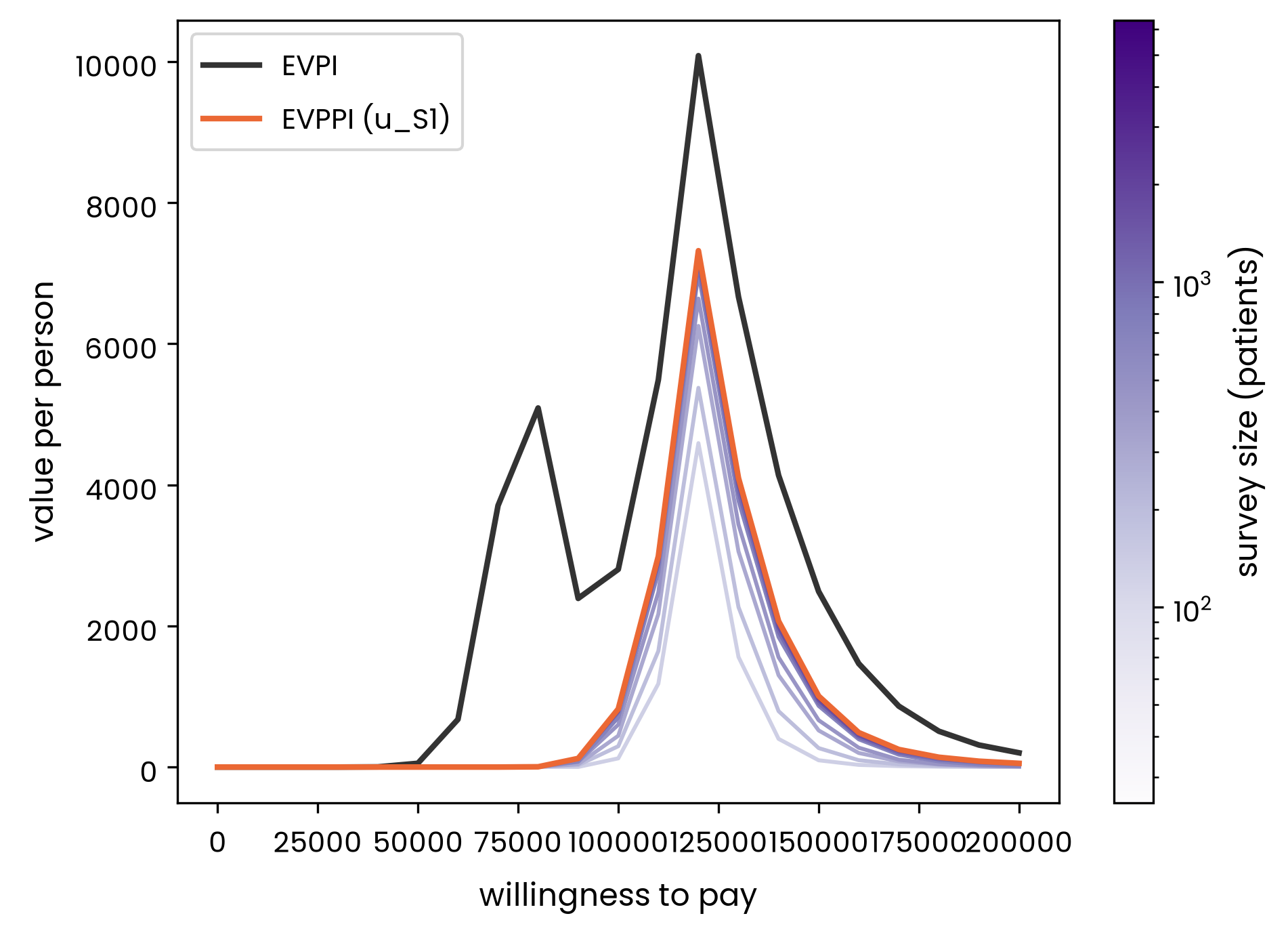
Expected net benefit of sampling (ENBS)
How many patients should the survey enroll? The expected net benefit of sampling (ENBS) answers that by multiplying the per-person EVSI by the population it would inform and discounting to a present value, then subtracting the survey’s cost. Suppose 2,000 patients enter the Sick state each year for 10 years, discounted at 3% a year, and each would benefit from a decision informed by the resolved utility. The survey costs a fixed 100,000 to set up plus 300 per participant. An ENBS at or above zero is the condition for running the survey; the size that maximizes it is the one worth funding.
i_wtp = int(np.where(grid == WTP)[0][0])
evsi = pd.Series({n: fan[n][i_wtp] for n in sizes})  # EVSI at the reference threshold
years = np.arange(10)
beneficiaries = 2_000 * (1.03 ** -years).sum()  # discounted future patients
cost = 100_000 + 300 * np.array(sizes)
enbs = pd.Series(beneficiaries * evsi.to_numpy() - cost, index=pd.Index(sizes, name="patients"))
best = enbs.idxmax()
print(f"optimal size: {best} patients, ENBS {enbs[best]:,.0f}")
enbs.round(0)
optimal size: 1600 patients, ENBS 13,399,952patients
25 2062662.0
50 5072873.0
100 7661816.0
200 10393951.0
400 12101950.0
800 13340125.0
1600 13399952.0
3200 13046084.0
6400 12383773.0
dtype: float64ENBS rises with survey size as long as the added precision is worth more than its cost, then falls once EVSI approaches the EVPPI ceiling and the survey keeps costing more per patient without resolving much further uncertainty.
ax = enbs.plot(marker="o", xlabel="survey size (patients)", ylabel="ENBS")
ax.axhline(0, color="0.6", lw=0.8);
ax.plot(best, enbs[best], "r*", ms=14);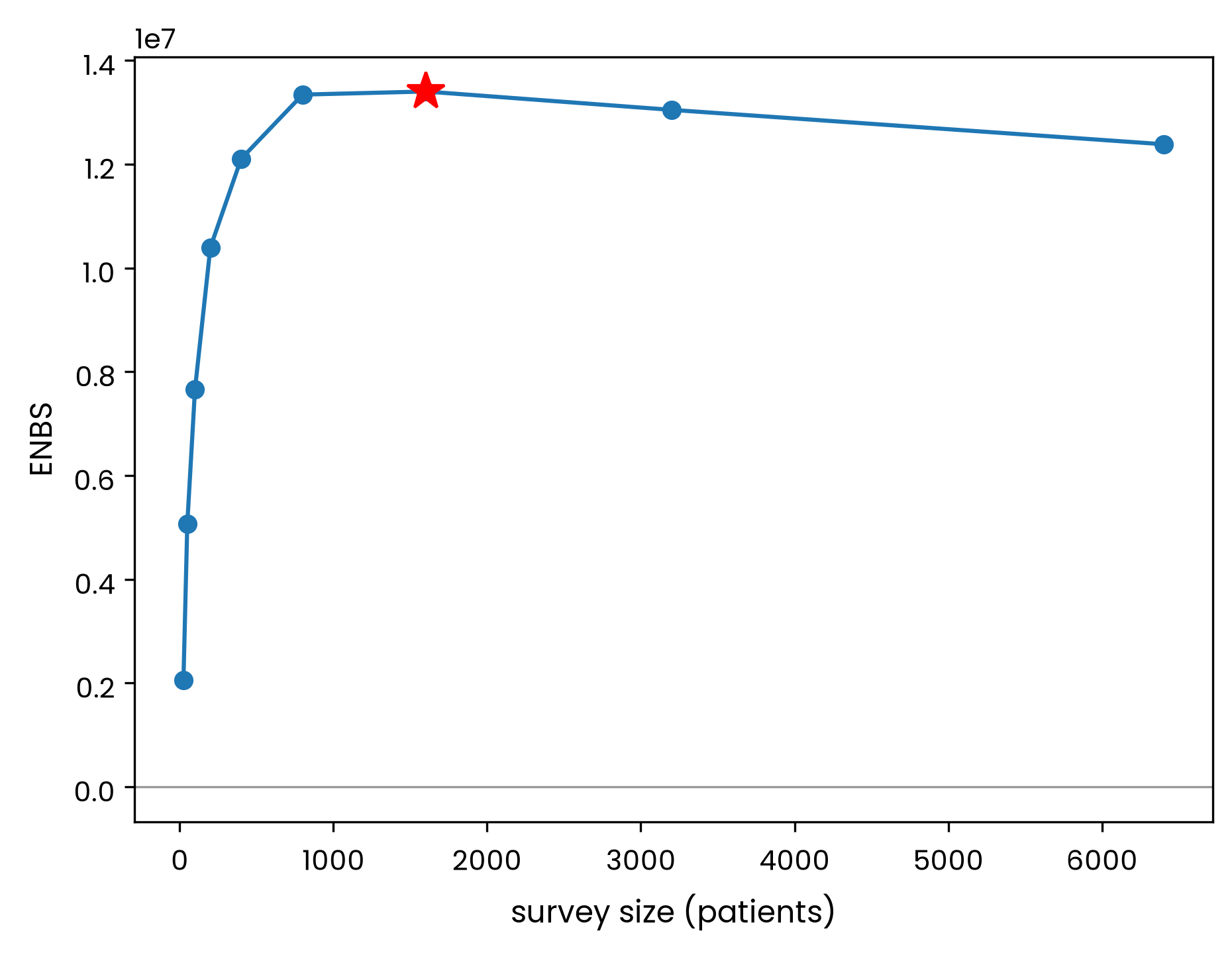
Keywords: value of information, VOI, EVPI, EVPPI, EVSI, expected value of perfect information, expected value of partial perfect information, expected value of sample information, health economics, Python