import numpy as np
import pandas as pd
from heormodel.models import CohortSpec, MarkovModel

STATES = ("healthy", "sick", "dead")
INTERVENTION = "natural_history"
N_CYCLES = 40
TARGET_CYCLES = (8, 16, 28)
TARGET_LABELS = [f"sick_c{cycle}" for cycle in TARGET_CYCLES]
BACKGROUND_MORTALITY = 0.01

CALIBRATED = ("p_HS", "p_SD")
BOUNDS = {"p_HS": (0.02, 0.20), "p_SD": (0.05, 0.35)}
TRUTH = {"p_HS": 0.08, "p_SD": 0.15}

def transitions_and_rewards(params, intervention):
    p_HS, p_SD = params["p_HS"], params["p_SD"]
    transition = np.array([
        [1.0 - p_HS - BACKGROUND_MORTALITY, p_HS, BACKGROUND_MORTALITY],
        [0.0, 1.0 - p_SD, p_SD],
        [0.0, 0.0, 1.0],
    ])
    return CohortSpec(transition, np.zeros(3), np.array([1.0, 0.8, 0.0]))

engine = MarkovModel(
    states=STATES, interventions=(INTERVENTION,),
    transitions_and_rewards=transitions_and_rewards,
    n_cycles=N_CYCLES, cycle_correction="none",
)Calibrating with ABC
Calibrate a parameter to observed data with approximate Bayesian computation, the first of four calibration tutorials that share one disease model.

This tutorial shows how to calibrate an unknown model parameter to observed data using approximate Bayesian computation (ABC), a method that infers parameters by simulating from the model and keeping the parameter sets whose output matches the data. It is the first of four calibration tutorials that share one disease model, so the posteriors can be compared across methods. Here the model is deterministic and the only uncertainty is in the data: the calibration target is a prevalence measured in a finite sample. It walks through examples/calibrate_abc.py and needs the calibration extra: uv pip install 'heormodel[calibration]'.
Calibration is the inverse of running a model. A model turns parameters into outputs; calibration starts from observed outputs and recovers the parameters consistent with them. The target is the Bayesian posterior, the prior reweighted by how well each parameter set reproduces the data, \(p(\theta \mid \text{data}) \propto p(\text{data} \mid \theta)\,p(\theta)\). ABC reaches it without writing down the likelihood \(p(\text{data} \mid \theta)\): it proposes parameters \(\theta\) from the prior, runs the model, and accepts the proposal when the simulated summary lands within a tolerance \(\varepsilon\) of the observed one,
\[\rho\big(S(\theta),\, S_\text{obs}\big) \le \varepsilon.\]
Successive rounds shrink \(\varepsilon\), so the accepted parameters approach the posterior.
Specifying the disease model
The model is a three-state cohort state-transition (Markov) model over Healthy, Sick, and Dead, run for 40 annual cycles from a healthy cohort. Two per-cycle transition probabilities are unknown and will be calibrated: the Healthy to Sick probability p_HS and the Sick to Dead probability p_SD. Background mortality from Healthy is held fixed.
The calibration reads three numbers from the cohort trace: the Sick-state prevalence at cycles 8, 16, and 28. An early, middle, and late reading of the Sick-state trajectory together separate the inflow probability p_HS from the outflow probability p_SD, which a single reading would confound.
def prevalence(params):
    """Sick-state prevalence the model predicts at the target cycles."""
    occupancy = engine.trace(pd.Series(params), INTERVENTION)["sick"].to_numpy()
    return np.array([occupancy[cycle] for cycle in TARGET_CYCLES])
Measuring the target in a finite sample
The target is not the prevalence itself but a measurement of it. Prevalence is estimated from a sample of people, and a sample of 1,000 carries a sampling error of about 1.5 percentage points at these values. The observed target is one such measurement: a count of how many of 1,000 people are in the Sick state, drawn once from the true prevalence with a fixed seed so the reading is reproducible. The model is deterministic, so this sampling error is the only uncertainty the calibration faces.
SURVEY_SIZE = 1_000
SURVEY_SEED = 20260718

true_prevalence = prevalence(TRUTH)
observed = np.random.default_rng(SURVEY_SEED).binomial(SURVEY_SIZE, true_prevalence) / SURVEY_SIZE
survey_se = np.sqrt(true_prevalence * (1 - true_prevalence) / SURVEY_SIZE)
pd.DataFrame({"true": true_prevalence, "observed": observed, "se": survey_se},
index=TARGET_LABELS).round(4)| true | observed | se | |
|---|---|---|---|
| sick_c8 | 0.2637 | 0.271 | 0.0139 |
| sick_c16 | 0.1958 | 0.210 | 0.0125 |
| sick_c28 | 0.0810 | 0.091 | 0.0086 |
The observed prevalences fall within about one standard error of the truth that generated them. Generating the target from known values, p_HS = 0.08 and p_SD = 0.15, gives the calibration a right answer to recover.
Running the calibration
abc_calibrate runs sequential Monte Carlo ABC. It needs three things: a simulator that turns a parameter set into the same quantities as the target, the priors to sample parameters from, and the observed target. The simulator mirrors the measurement, returning a fresh sample of the model’s prevalence rather than the prevalence itself, so ABC recovers the parameters given a noisy reading and carries the sampling error into the posterior. The acceptance threshold anneals down to half the single-sample scale, which sharpens the posterior below the width one sample would give, because the simulator draws its own sample with the same error as the data.
import os
os.environ["ABC_LOG_LEVEL"] = "WARNING"  # quiet pyabc's per-population logging

from heormodel.calibrate import abc_calibrate
from heormodel.params import Uniform

sim_rng = np.random.default_rng(2024)

def simulator(params):
    survey = sim_rng.binomial(SURVEY_SIZE, prevalence(params)) / SURVEY_SIZE
    return dict(zip(TARGET_LABELS, survey))

epsilon = 0.5 * float(np.sqrt((true_prevalence * (1 - true_prevalence) / SURVEY_SIZE).sum()))
result = abc_calibrate(
    simulator,
    priors={name: Uniform(*BOUNDS[name]) for name in CALIBRATED},
    observed=dict(zip(TARGET_LABELS, observed)),
    population_size=400,
    max_populations=15,
    min_epsilon=epsilon,
    n_posterior=3_000,
    seed=1,
)
posterior = result.posterior
print(f"{result.n_populations} populations, final epsilon {result.final_epsilon:.4f}")
11 populations, final epsilon 0.0093The result carries the posterior as an equally weighted draw matrix, the same form a probabilistic sensitivity analysis consumes, so a calibrated parameter feeds the rest of a model the same way a literature parameter does. Its mean recovers the values that generated the target.
summary = pd.DataFrame({
    "truth": [TRUTH[name] for name in CALIBRATED],
    "posterior_mean": posterior.mean().reindex(CALIBRATED).to_numpy(),
    "posterior_sd": posterior.std().reindex(CALIBRATED).to_numpy(),
}, index=list(CALIBRATED))
summary.round(4)| truth | posterior_mean | posterior_sd | |
|---|---|---|---|
| p_HS | 0.08 | 0.0793 | 0.0059 |
| p_SD | 0.15 | 0.1400 | 0.0060 |
The posterior means are within about a standard error of the truth, and the standard deviations show how precisely a sample of 1,000 constrains each parameter. Overlaying the marginal posteriors on the true values shows the same recovery.
import matplotlib.pyplot as plt

fig, axes = plt.subplots(1, len(CALIBRATED), figsize=(9, 3.5))
for axis, name in zip(axes, CALIBRATED):
    axis.hist(posterior[name], bins=40, density=True, alpha=0.6, color="#2a6f97")
    axis.axvline(TRUTH[name], color="black", linestyle="--", linewidth=1, label="truth")
    axis.set_xlabel(name)
    axis.set_yticks([])
axes[0].set_ylabel("posterior density")
axes[-1].legend(fontsize=8)
fig.tight_layout()
plt.show()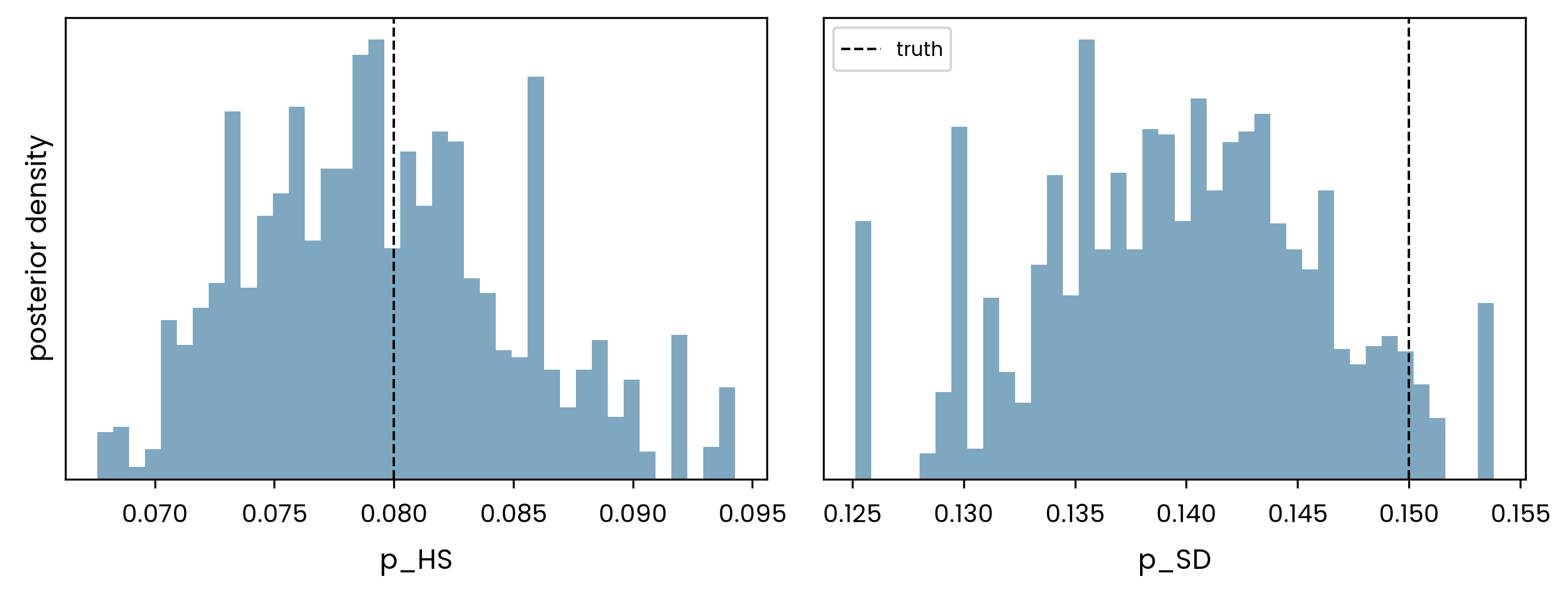
The cost is the run count. Reaching this posterior took several thousand model evaluations, because every accepted parameter set in every population is a model run and most proposals are rejected. That cost is bearable when the model is a cohort trace that runs in milliseconds. When a single run is slow, it becomes the constraint, which the surrogate tutorial addresses.
Next: the simulation-based inference tutorial calibrates the same model to the same target with a different method, and reaches the same posterior.